Calculating Low Power Wide Area Network End Node Battery Longevity
LPWAN end node longevity relies on dynamic state-machine energy integration multiplied by chemical passivation and thermal capacity derating factors.

States
A low-power wide-area network end node spends over ninety-nine percent of its life asleep, but total battery life depends on the sum of discrete power states, state transitions, and peripheral startup overheads. Calculating how long a node will survive starts with mapping the complete finite state machine of the radio and microcontroller. Modes range from deep sleep with low leakage, real-time clock retention sleep, active processing, and peripheral data acquisition, to synthesizer lock, power amplifier transmit bursts, and receiver windows.
Each state draws a specific current for a duration dictated by firmware execution and silicon physics.
Sleep current forms the absolute baseline of battery drain. Silicon vendors report leakage under ideal lab conditions with core rails off, RTCs disabled, and ambient temperature fixed at twenty-five degrees Celsius. In field deployments, internal low-dropout regulators remain active to power retention RAM, while internal real-time clocks run continuously to manage wake-up timers.
Leakage current escalates non-linearly with temperature, doubling roughly every ten degrees Celsius rise in silicon junction temperature. A micro-controller rated at 800 nanoamps of sleep current at ambient conditions draws over four microamps inside an unshaded outdoor enclosure at sixty degrees Celsius. This baseline sleep current runs perpetually, consuming substantial mAh capacity across multi-year operating horizons regardless of radio activity.
Wake-up transitions add transient energy costs that datasheets often smooth over in average power figures. Leaving sleep forces the power management unit to stabilize internal voltage rails, ungate system clocks, and wait for high-frequency crystal oscillators to lock. A high-speed crystal oscillator takes several milliseconds to settle its output amplitude and frequency tolerance.
During this phase, the microcontroller runs at full active current without executing application code, spending energy simply reaching a usable state. Internal flash memory power-up delays extend this further while charge pumps reach operating voltages before reading code instructions.
| Operational State | Sub-GHz Direct Sequence (868/915 MHz) | Sub-GHz Chirp Spread Spectrum | Cellular LPWAN NB-IoT (Band 8/20) | Cellular LPWAN LTE-M (Band 3/8) |
|---|---|---|---|---|
| Deep Sleep / PSM Current | 0.8 µA | 1.2 µA | 3.1 µA | 4.5 µA |
| Synthesizer Lock Duration | 120 µs | 180 µs | 4.2 ms | 3.8 ms |
| Active Transmit Current (+14 dBm) | 28 mA | 32 mA | 110 mA | 140 mA |
| Active Transmit Current (+20/23 dBm) | 82 mA | 125 mA | 220 mA | 265 mA |
| Receiver Mode Current | 9.5 mA | 11.2 mA | 46 mA | 54 mA |
| Cold Join / Registration Overhead | 1.2 mWh | 1.8 mWh | 45 mWh | 38 mWh |
Active sensor acquisition states introduce additional current steps prior to radio engagement. Analog-to-digital converters, sensor excitation bias networks, internal reference voltages, and external bus pull-up resistors demand energy before data packet construction begins. Powering a wheatstone bridge strain gauge or an optical particle counter creates milliamp-level current spikes lasting tens to hundreds of milliseconds.
Firmware that leaves sensor power rails enabled during micro-controller sleep states destroys battery capacity through sneak paths and un-isolated input pins.
Holding sleep leakage current below two microamps across operational temperature swings forms the absolute floor of long-term battery survival.
Radio frequency lock sequence overhead represents a fixed energy tariff incurred on every transmission event. The local oscillator frequency synthesizer must lock onto the target channel, calibrate internal voltage-controlled oscillators, and adjust image rejection filters before the power amplifier enables its output stage. Disregarding the synthesizer settling phase in energy accounting undercounts per-transmission energy consumption by five to fifteen percent depending on payload brevity.
The current drawn during frequency lock matches or exceeds receiver current levels, making frequent short transmissions disproportionately expensive in total energy balance.
Miscalculating the duration or current draw of any individual state in the finite state machine distorts total longevity estimates, leading to premature field exhaustion long before theoretical battery capacity ratings expire.

Chemistry
Primary batteries engineered for wireless nodes use chemistries that trade peak power delivery for energy density and low self-discharge. Lithium Thionyl Chloride (Li-SOCl2) is standard for sub-GHz deployments because of its nominal 3.6 volts and annual self-discharge rate under one percent in clean storage. Lithium Manganese Dioxide (Li-MnO2) operates at 3.0 volts and provides higher pulse currents without severe passivation delays, which suits cellular LPWAN nodes taking frequent high-current transmission bursts.
Liquid cathode chemistries rely on solid-electrolyte interface dynamics that directly alter available capacity under pulsed loads.
Passivation both protects Lithium Thionyl Chloride cells and complicates their use. A thin insulating film of lithium chloride forms on the metallic lithium anode while idle, preventing direct reaction with the thionyl chloride liquid cathode. This film keeps self-discharge to fractions of a percent per year.
When the node shifts from microamp sleep to milliamp transmission, the passivation layer acts as internal electrical resistance, causing a brief voltage dip known as voltage delay. If terminal voltage drops below the power management IC brownout threshold, the microcontroller resets before transmitting a single symbol.
Disrupting this passivation layer requires a controlled pulse sequence to break up the lithium chloride structure mechanically. Firmware routines periodically wake the node to draw moderate current pulses, spending a little active energy solely to keep internal cell impedance low. Cold ambient temperatures worsen passivation resistance and slow down its breakdown during pulses.
Deploying nodes into sub-zero municipal or refrigeration settings requires testing cell voltage under cold pulsed loads rather than relying on room-temperature discharge curves.
Internal cell impedance increases linearly as depth of discharge progresses, reducing maximum deliverable pulse current near end-of-life. A fresh cell presenting two ohms of internal DC resistance exhibits over twenty ohms after eighty percent of its rated capacity exhausts. Pulsing a twenty-ohm cell at one hundred milliamps generates a two-volt internal IR drop across the battery terminal itself.
The terminal voltage under load drops from 3.6 volts to 1.6 volts, instantly tripping micro-controller low-voltage lockouts despite substantial chemical energy remaining inside the cell casing.
Dynamic internal cell impedance increases near end of life, causing severe terminal voltage drop under high radio transmit pulses.
Capacity derating curves reveal that nominal milliamp-hour ratings printed on battery casings apply only under ultra-low continuous discharge currents at twenty-five degrees Celsius. High peak transmission currents reduce total accessible capacity by causing localized ion depletion within the cell matrix and premature internal heating. Discharge curves published by primary battery manufacturers reflect constant current continuous loads, which fail to simulate the high-crest-factor pulsed current profiles characteristic of LPWAN transmissions.
Pulsed loads reduce usable cell capacity by ten to thirty percent relative to datasheet continuous discharge specifications.
Self-discharge accelerates under thermal stress. Higher temperatures increase reaction kinetics across the lithium surface, breaking down the passivation film and raising baseline self-discharge from one percent per year at twenty-five degrees Celsius to over five percent at sixty degrees Celsius. Nodes mounted on rooftops or uninsulated industrial equipment suffer compound losses: elevated silicon leakage current combined with accelerated battery self-discharge.
Battery vendors often point to room-temperature capacity ratings during performance disputes, attributing field dropouts to thermal cycling beyond standard testing bounds.

Airtime
Airtime is the primary driver of active radio energy consumption, converting transmit power and modulation duration directly into milliwatt-hours of battery drain. Transmit duration scales with payload size, channel coding rates, preamble length, and modulation parameters. In sub-GHz Chirp Spread Spectrum systems, airtime doubles with nearly every increment in spreading factor.
A twenty-byte application payload sent at Spreading Factor 7 on a 125 kHz channel bandwidth requires approximately forty-six milliseconds of on-air time. The same payload transmitted at Spreading Factor 12 requires over one thousand three hundred milliseconds, expanding active transmit energy by a factor of nearly twenty-eight for identical data payload content.
Cellular LPWAN protocols introduce complex temporal framing structures that decouple application payload size from total active RF airtime. Narrowband IoT utilizes Narrowband Physical Uplink Shared Channel allocations that scale from single-tone 15 kHz subcarrier spacing up to multi-tone formats. A node operating under deep coverage extension mode executes up to 128 or 256 physical layer repetitions of every subframe to build energy at the base station receiver.
Repeating a subframe two hundred and fifty-six times transforms a short sixty-millisecond uplink transmission into a multi-second continuous power amplifier burn, exhausting several Coulombs of battery charge in a single packet transmission event.
Protocol framing adds substantial structural overhead before application bytes enter the physical layer frame. MAC headers, device addresses, frame counters, cryptographic authentication codes, and physical layer preambles add mandatory bytes to every packet. Short application payloads bear high overhead ratios: transmitting a two-byte temperature reading takes at least a twenty-three byte MAC frame in LoRaWAN, while cellular protocols wrap data in IP headers, UDP wrappers, and DTLS envelopes that expand the packet by fifty to one hundred bytes.
Which Protocol Mechanisms Exert the Highest Airtime Energy Penalty?
Downlink reception windows impose mandatory receiver energization periods following every uplink transmission. In class A LoRaWAN nodes, the receiver enables its baseband circuitry for two distinct RX windows at fixed delays after uplink completion. The baseband processor must remain fully powered while checking for preamble symbols on the designated channel.
If a preamble is detected, the radio stays active to process the complete downlink frame, consuming receiver current for tens of milliseconds. Unsynchronized cellular idle modes require nodes to process physical downlink control channels during Extended Discontinuous Reception (eDRX) paging cycles, forcing periodic active receiver processing to maintain network paging synchronization.
Regulatory band plans establish legal ceilings on radio airtime that directly affect firmware protocol architecture and transmission cadences. ETSI EN 300 220 rules governing European sub-GHz ISM bands enforce strict duty-cycle limits of 0.1 percent or 1.0 percent across specific channel sub-bands, limiting maximum continuous transmission time per hour. Operating under a one percent duty-cycle restriction caps total aggregate airtime to thirty-six seconds per hour.
FCC Part 15.247 rules governing North American 915 MHz allocations replace duty-cycle limits with maximum dwell time rules or hybrid frequency hopping provisions that dictate minimum channel counts and maximum channel occupancy periods.
| Protocol and Operating Parameter | Physical Data Rate | Total Frame Airtime | Peak Transmit Current (+14/+20 dBm) | Energy Spent Per Transmission |
|---|---|---|---|---|
| LoRaWAN EU868 SF7 (125 kHz) | 5470 bps | 46.3 ms | 32 mA @ 3.3V | 0.0049 mWh |
| LoRaWAN EU868 SF10 (125 kHz) | 980 bps | 370.7 ms | 32 mA @ 3.3V | 0.0391 mWh |
| LoRaWAN EU868 SF12 (125 kHz) | 250 bps | 1318.9 ms | 125 mA @ 3.3V (+20 dBm) | 0.5440 mWh |
| NB-IoT Standalone (1 Repetition, Multi-Tone) | 15 kbps | 120.0 ms | 110 mA @ 3.3V | 0.0435 mWh |
| NB-IoT Extended Coverage (64 Repetitions) | 0.2 kbps | 4800.0 ms | 220 mA @ 3.3V (+23 dBm) | 3.4848 mWh |
| LTE-M Cat-M1 (1 Repetition, 6 Blocks) | 150 kbps | 15.0 ms | 140 mA @ 3.3V | 0.0069 mWh |
Network acknowledgment policies severely compound total energy expenditure when operating over lossy wireless channels. Unacknowledged transmissions burn energy purely for uplink airtime. Acknowledged transmissions mandate active receiver window processing, processing overhead for downlink parsing, and retransmission retry mechanisms when acknowledgments fail to arrive.
A node configured for eight retransmission attempts over a degraded channel will retransmit its payload eight times before declaring link failure, consuming eight times the baseline transmission energy while simultaneously escalating transmit power or spreading factors.
Commercial network service level agreements often mandate explicit acknowledgment mechanisms and dynamic link fallback routines that directly modify local firmware transmission parameters during link degradation events.
Fade
Path loss dictates RF power requirements, linking propagation mechanics directly to battery drain. In ideal free space, power density falls off with the square of distance. Real indoor, subterranean, and urban settings introduce obstacles, attenuation, and multipath interference that push path loss exponents to between 3.0 and 4.8.
High path loss forces nodes to boost transmit power or switch to lower-rate modulation to maintain packet reception at the gateway.
Adaptive Data Rate (ADR) algorithms attempt to optimize node airtime and transmit power based on historical link quality statistics collected at the network server. When signal-to-noise ratios (SNR) and received signal strength indicators (RSSI) exceed base threshold requirements, the network commands the node to reduce transmit power or decrease spreading factors, conserving battery capacity. Conversely, when path loss increases due to seasonal vegetation changes, architectural modifications, or physical movement, the network forces the node up to higher spreading factors and maximum RF output power levels.

Which Propagation Variables Accelerate Battery Drain Fastest?
Fade margins act as safety buffers to preserve link reliability as environmental conditions shift. Multipath reflections cause Rayleigh fading, dropping signals by over thirty decibels in localized spots. Obstructions create log-normal shadow fading over larger areas.
Maintaining a ninety-nine percent packet delivery ratio requires holding a fade margin ten to twenty decibels above receiver sensitivity. Operating without that margin leads to dropped packets and retry cycles that rapidly deplete the battery.
Antenna mismatch and body loss convert RF power into heat before electromagnetic energy leaves the node enclosure. Placing an end node against high-permittivity materials such as concrete walls, metallic piping, or wet soil detunes the printed circuit board antenna, shifting its resonant frequency away from the operating band. Antenna impedance mismatch causes significant power reflection back into the transmitter power amplifier, decreasing effective radiated power (ERP) while increasing current draw.
A six-decibel antenna detuning loss cuts effective radiated power by seventy-five percent, forcing the node to compensate by shifting from SF7 to SF9 or raising power amplifier output from +14 dBm to +20 dBm.
- Link Budget Margin Calculation determines the baseline path loss headroom by comparing maximum transmitter power plus antenna gains against receiver sensitivity and required fade margins across target deployment terrains.
- Environmental Attenuation Mapping identifies fixed RF losses introduced by building walls, foil-backed insulation, metallic ducting, subterranean soil moisture levels, and dense structural concrete enclosures.
- Antenna Detuning Profiling measures voltage standing wave ratio shifts and efficiency degradation resulting from housing plastics, battery proximity, mounting bracket materials, and physical installation surroundings.
- Adaptive Rate Convergence Audit verifies how rapidly network server optimization algorithms restore optimal modulation parameters and transmit power levels following transient RF interference events.
- Retransmissions Envelope Analysis establishes worst-case energy budgets by modeling frame error rates against retransmission trial caps under severely degraded link margin conditions.
Subterranean deployments present extreme path loss conditions due to soil moisture absorption and dielectric attenuation. RF signals operating in the 868/915 MHz bands experience attenuation rates between ten and one hundred decibels per meter through wet topsoil. End nodes deployed in underground utility vaults or soil moisture monitoring arrays must utilize maximum power settings and highest spreading factors continuously.
Operating continuously at maximum link capacity converts every transmission into a peak-energy event, reducing multi-year service life down to months unless transmission cadences scale down proportionally.
Antenna impedance detuning against concrete or metal surfaces converts transmit power into heat, doubling energy spent per delivered byte.
How does dynamic seasonal foliage attenuation alter long-term adaptive data rate distributions across multi-year node field deployments?


Model
Estimating LPWAN battery life requires an energy accounting model that integrates discrete electrical currents over time, factors in battery chemistry degradation, and applies mathematical deratings for self-discharge and environmental stress. Simple calculations dividing capacity by average current give overly optimistic figures that fail in the field. Reliable estimates combine finite state energy summation with non-linear capacity reduction factors.
The total energy consumed during one complete operational period, Ecycle, expressed in milliamp-seconds (mAs) or Coulombs, is defined by summing the products of current draw Ik and duration tk for every state k within the state machine:
Ecycle = sumk=1N (Ik · tk) + Etrans
Where Ik represents current in milliamps, tk represents duration in seconds, and Etrans accounts for total energy spent during voltage rail and oscillator stabilization transitions between states. The daily energy consumption Edaily in milliamp-hours (mAh) incorporates active cycle frequency per day M, active event retransmission factor R, and background micro-controller sleep current Isleep integrated across twenty-four hours:
Edaily = left( fracM · R · Ecycle3600 right) + left( Isleep · 24 right)
Total accessible battery capacity Caccessible in mAh is calculated by applying derating coefficients to the nominal rated cell capacity Cnominal:
Caccessible = Cnominal · Ktemp · Kpulse · Kaging
Where Ktemp models thermal capacity reduction, Kpulse accounts for pulse discharge efficiency losses, and Kaging accounts for chemical manufacturing variance and structural breakdown over time. Annual chemical self-discharge loss Cself expressed in mAh per year is calculated using the baseline self-discharge rate Sanνal modified by temperature acceleration factor αtemp:
Cself = Caccessible · (Sanνal · αtemp)
The final predicted operational longevity Tyears in calendar years derives from balancing total accessible capacity against combined daily operational consumption and annual self-discharge losses:
Tyears = fracCaccessibleleft( Edaily · 365.25 right) + Cself
Worked Longevity Calculation Example
To demonstrate the model, consider a practical outdoor industrial tracking node utilizing a sub-GHz Chirp Spread Spectrum radio powered by a single Lithium Thionyl Chloride (Li-SOCl2) ER14505 AA-size cell. The cell carries a nominal capacity rating Cnominal = 2400 mAh at twenty-five degrees Celsius. The node operates outdoors under thermal variations ranging from negative ten to forty degrees Celsius, yielding Ktemp = 0.88.
Peak radio pulse currents of 120 mA introduce pulse losses represented by Kpulse = 0.85, while aging allowance is set to Kaging = 0.95.
Caccessible = 2400 · 0.88 · 0.85 · 0.95 = 1705.4 mAh
The device transmits one twenty-byte payload every fifteen minutes (M = 96 transmissions per day). Network radio conditions force a mix of Spreading Factor 9 (80% of transmissions) and Spreading Factor 12 (20% of transmissions) under Adaptive Data Rate adjustment. The link degradation model predicts an average retransmission factor R = 1.15 to account for lost packet retries.
| State Phase (k) | SF9 Current (Ik) | SF9 Duration (tk) | SF12 Current (Ik) | SF12 Duration (tk) |
|---|---|---|---|---|
| Sensor Initialization and Read | 4.2 mA | 45 ms | 4.2 mA | 45 ms |
| Radio Synthesizer Lock | 9.0 mA | 2.5 ms | 9.0 mA | 2.5 ms |
| Uplink RF Transmission | 45.0 mA (+14 dBm) | 185.0 ms | 125.0 mA (+20 dBm) | 1318.9 ms |
| RX1 Preamble Listen Window | 11.2 mA | 40.0 ms | 11.2 mA | 40.0 ms |
| Processing and Memory Write | 6.5 mA | 12.0 ms | 6.5 mA | 12.0 ms |
Calculating cycle energy spent for an SF9 transmission event:
ESF9 = (4.2 · 0.045) + (9.0 · 0.0025) + (45.0 · 0.185) + (11.2 · 0.040) + (6.5 · 0.012) = 9.062 mAs
Calculating cycle energy spent for an SF12 transmission event:
ESF12 = (4.2 · 0.045) + (9.0 · 0.0025) + (125.0 · 1.3189) + (11.2 · 0.040) + (6.5 · 0.012) = 165.813 mAs
Weighted average cycle energy Ecycle considering modulation distribution:
Ecycle = (0.80 · 9.062) + (0.20 · 165.813) = 40.412 mAs
Sleep current leakage averages Isleep = 0.0022 mA (2.2 µA) across the outdoor temperature profile. Daily energy calculation Edaily:
Edaily = left( frac96 · 1.15 · 40.4123600 right) + (0.0022 · 24) = 1.2404 + 0.0528 = 1.2932 mAh/day
Annual self-discharge rate Sanνal = 0.01 (1% per year), with outdoor temperature acceleration factor αtemp = 1.8, yielding 1.8% anνal loss:
Cself = 1705.4 · 0.018 = 30.697 mAh/year
Applying values into the final longevity equation:
Tyears = frac1705.4(1.2932 · 365.25) + 30.697 = frac1705.4472.341 + 30.697 = frac1705.4503.038 = 3.39 years
This worked result reveals that despite theoretical marketing claims promising ten-year operation from a 2400 mAh cell, real-world outdoor temperature derating, periodic high-power retransmissions, and modulation mix reduce actual field service life to 3.39 years.
Summing microamp-seconds across real-world state transitions yields reliable longevity figures, whereas dividing nominal milliamp-hour ratings by average current produces field failures.

Bench
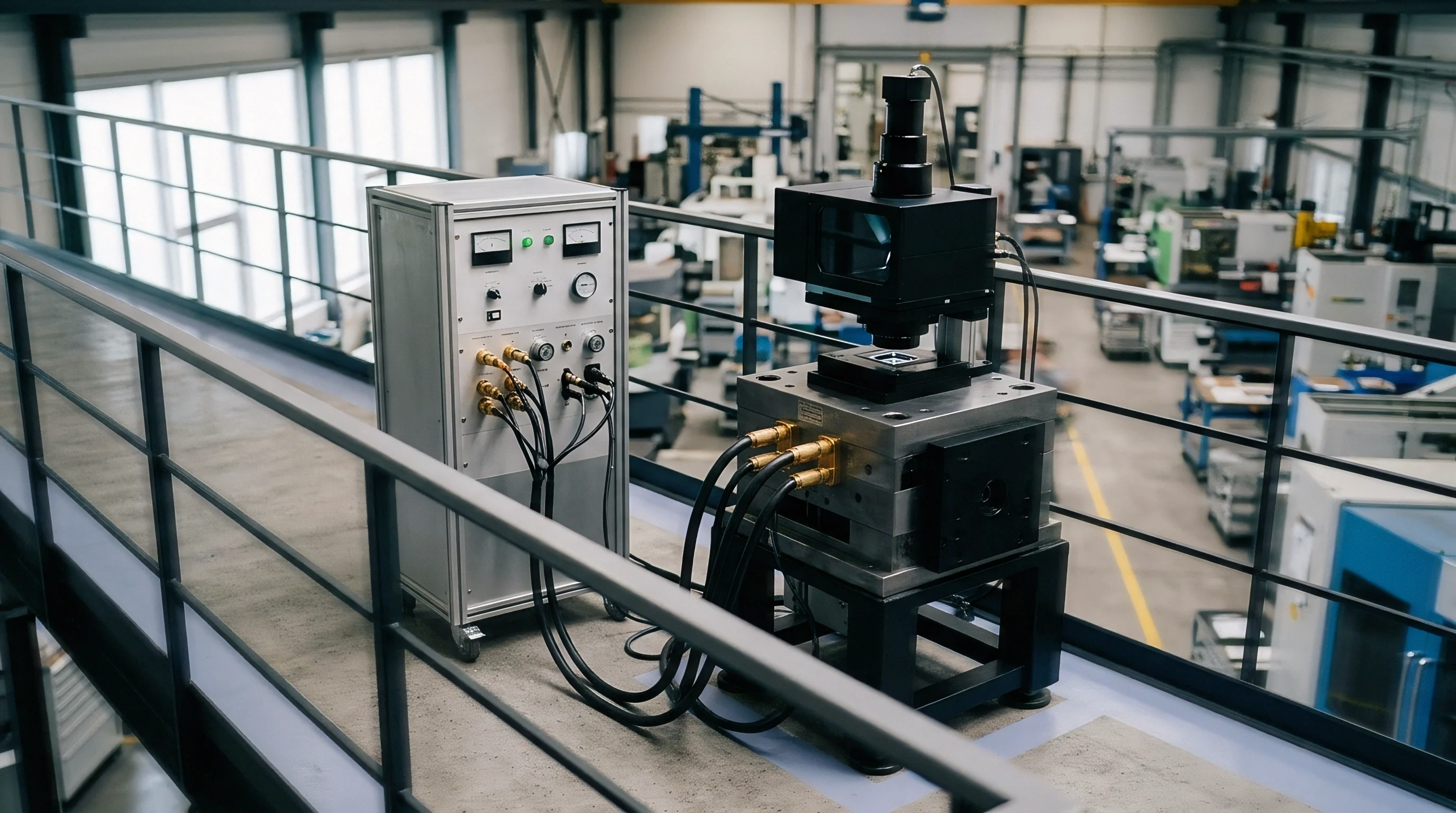
Laboratory validation of end node energy profiles requires measurement instruments capable of capturing dynamic current spans across six orders of magnitude. Standard multimeters lack the bandwidth and auto-ranging speed to measure a jump from a two-hundred-nanoamp sleep state to a two-hundred-milliamp pulse. Switched-shunt power analyzers and specialized Coulomb counters use transimpedance amplifiers and high-speed ADCs sampling at up to one hundred kilosamples per second to capture fast transients without introducing burden voltage errors.
Burden voltage is the drop created across an instrument’s current-sensing resistor. If a meter inserts a high sense resistance to measure microamp sleep current, a sudden two-hundred-milliamp radio transmit pulse causes an immediate voltage drop across the sensor. This artificial drop lowers supply voltage at the node terminals, triggering brownout resets that would not occur on battery power.
Dynamic auto-ranging shunt analyzers switch sensing resistors in sub-microsecond timeframes to keep burden voltage low across all operating currents.
Environmental thermal profiling validates chemical battery performance and silicon leakage currents under accelerated climate conditions. Placing the node and its target primary cell inside a programmable thermal chamber allows testing across the full target industrial operating envelope, such as negative forty degrees to eighty-five degrees Celsius. Automated test scripts trigger continuous transmit cycles while monitoring cell terminal voltage drop on an oscilloscope, capturing the exact voltage delay curve caused by chemical passivation breakdown under cold-temperature pulse conditions.
Hardware-in-the-loop (HIL) test setups combine programmable RF attenuators, network emulators, and dynamic current profilers to simulate dynamic field conditions deterministically. By stepping RF channel attenuation across a controlled matrix, test engineers force the end node to adjust transmit power levels, alter spreading factors, execute retransmission retries, and trigger rejoin procedures under repeatable lab conditions. Integrating automated current integration software into the test loop directly measures Coulomb consumption for each protocol response state, providing empirical data to calibrate mathematical energy models.
Continuous integration bench testing verifies that firmware updates do not introduce energy regression bugs into production devices. A single unhandled GPIO pin floating in an undefined logic state during sleep mode can increase node sleep current by tens of microamps, reducing multi-year battery life down to several months. Automated nightly build regression setups execute standardized ten-minute operational scripts, continuously logging microamp-second totals to instantly flag software commits that compromise node energy budgets before code enters production release channels.
Long-term qualification profiles measure quiescent drain currents over multi-week hold intervals to detect subtle micro-controller peripheral leakages and power rail cross-talk. Connecting current profiling probes to prototype batches inside climate chambers reveals slow thermal drift parameters, dielectric breakdown inside filtering capacitors, and memory retention power stability. Empirical laboratory verification replaces analytical capacity assumptions with measured charge figures, establishing traceable verification dossiers required before signing high-volume hardware procurement commitments.