Minimum Volume Floor Calculation under Fluctuating Contract Manufacturing Demand
Calculate minimum volume floors by dividing fixed line overhead by unit contribution margin adjusted for first pass yield and verified volatile demand.


Capacity
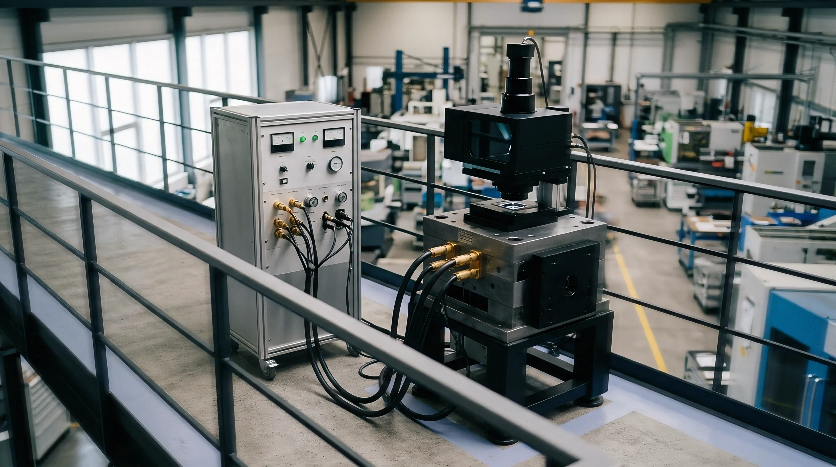
SMT Machine Overhead and Fixed Cost Recovery
Assembly facilities price production runs around machine utilization and overhead recovery. Surface-mount equipment depreciates on fixed accounting schedules regardless of board assembly volume. A pick-and-place line costing two million dollars depreciates across five years, creating a continuous hourly fixed overhead burden.
Factory operations allocate this capital expense alongside facility rent, environmental control, nitrogen supply, and indirect supervisory labor across planned machine operating hours.
When a customer commits to monthly manufacturing volume, the contract manufacturer reserves specific line hours based on expected component placement speeds and circuit board complexity. Machine rate models divide total factory overhead by available production hours, typically assuming an operating efficiency factor between seventy-five and eighty-five percent. If demand drops, these reserved line hours sit idle and fixed depreciation costs go unabsorbed, rapidly squeezing margins.
SMT production lines incur fixed depreciation charges between seventy-five and one hundred twenty dollars per hour regardless of active board assembly rate.
Unit pricing models assume full overhead absorption across agreed quantities. A quotation specifying ten dollars per assembled board might allocate three dollars to direct raw materials, two dollars to direct labor, four dollars to fixed overhead recovery, and one dollar to factory margin. If actual production volume falls by fifty percent, the four-dollar fixed overhead burden doubles per unit produced.
Contract manufacturers cannot absorb this margin compression without commercial compensation mechanisms.

Labor Allocation under Shift Adjustments
Technicians and line operators represent semi-fixed expenses during short demand drops. Specialist process engineers, quality control inspectors, and surface-mount operators cannot undergo immediate layoff during temporary volume contractions. Reassigning staff to alternate customer lines requires recalibration time and cross-training validation, creating unrecoverable labor friction.
Short-term demand dips force assembly facilities to maintain staffing levels while unit output declines, driving up direct labor costs per finished assembly during low-volume quarters. The failure to establish clear volume baselines leaves the buyer vulnerable to sudden quote revisions, surcharges, or retroactive price tier adjustments.


Floor

Defining Baseline Order Commitments
Contract manufacturing agreements use baseline volume thresholds to secure machine availability. A minimum volume floor establishes the absolute quantity of product a buyer guarantees to purchase or compensate within a specified contract window. This baseline protects the factory from unabsorbed overhead while providing the buyer with reserved production capacity and locked tier pricing.
Negotiating volume baselines involves balancing historical demand variance against factory operational constraints. The floor does not represent the forecasted mean demand; rather, it defines the operational break-even point where factory overhead recovery satisfies the master services agreement. Volume floors usually range between sixty and eighty percent of the nominal rolling forecast.
- Assess historical order variance across the previous four quarters to establish the baseline demand distribution.
- Extract fixed factory overhead figures from unit quotations to determine hourly line depreciation charges.
- Calculate the minimum unit threshold where factory overhead absorption covers fixed machine costs.
- Establish quarterly volume reconciliation terms with explicit financial adjustment formulas.
- Draft raw material purchase liabilities to separate component holding costs from board assembly charges.

Component Holding Liabilities and Buffer Allocation
Raw material inventory liabilities accumulate when purchase orders fall below forecasted projections. Contract manufacturers procure active components, printed circuit boards, and custom magnetics based on long-lead material authorizations. When finished goods assembly drops below the volume floor, component stock sits in factory bonded storage, tying up working capital and incurring inventory holding charges.
Holding charges typically run between one and one point five percent per month on total idle component stock value. Agreements assign this financial responsibility directly to the buyer when order volumes fall below agreed thresholds.
Standard electronics manufacturing agreements assign raw material liability to the buyer sixty days after purchase order cancelation or forecast drop.
Clear volume commitments determine the ownership boundary for custom components, end-of-life silicon, and raw materials ordered under extended vendor lead times. Section 4.2 of the standard electronics assembly agreement specifies that the buyer assumes full financial ownership of all non-cancellable, non-returnable materials procured to support agreed minimum volume floors.


Arithmetic

Mathematical Derivation of Fixed Cost Absorption
Establishing a mathematically sound volume baseline requires separating fixed overhead from variable assembly expenditures. Fixed overhead includes equipment depreciation, facility overhead, indirect supervision, and software licensing. Variable expenses encompass direct labor, solder paste, process nitrogen, protective packaging, and scrap allowances.
Consider the core variables in the floor derivation formula:
Let F represent monthly fixed facility overhead allocated to the reserved line.
Let L represent direct hourly labor rate assigned to active production.
Let R represent board throughput rate in units per hour.
Let P represent contracted unit price paid by the buyer.
Let M represent bill of materials direct unit cost.
Let Vf represent the minimum monthly volume floor in units.
The unit price covers direct materials, direct labor, overhead allocation, and target profit margin:
P = M + (L / R) + (F / Vnominal) + Marginunit
When actual monthly volume Vactual drops below Vnominal, total fixed overhead F remains unchanged. The unabsorbed overhead delta U equals:
U = F – (Vactual × (F / Vnominal))
To establish the minimum volume floor Vf where the factory recovers total fixed costs without generating operational losses, solve for the volume that yields zero unabsorbed overhead:
Vf = F / (P – M – (L / R))
Factoring first-pass assembly yield Y into the formulation adjusts the effective unit material and labor cost. The modified minimum volume floor equation becomes:
Vf = F / (P – (M / Y) – (L / (R × Y)))

Worked Floor Calculation for Volatile Orders
Consider an OEM contracting monthly printed circuit assembly across a volatile four-quarter window. The manufacturing partner dedicates one high-speed surface-mount placement line operating on a single eight-hour shift, twenty days per month (160 line hours monthly).
Assumed operational parameters for the assembly run:
- Allocated Fixed Line Overhead total monthly equipment depreciation, facility rent, and engineering support equals 24,000 dollars.
- Contracted Unit Price charged to the OEM per assembled circuit board equals 45 dollars.
- Direct Raw Material Cost billed per finished assembly equals 28 dollars.
- Direct Line Labor Cost fully burdened hourly rate for three line operators equals 90 dollars per hour total.
- Placement Line Throughput verified assembly speed equals 20 units per hour.
- First Pass Yield Rate verified factory test output rate equals 95 percent (0.95).
Step 1: Calculate direct labor cost per unit under yield factors.
Laborunit = 90 / (20 × 0.95) = 4.74 dollars
Step 2: Calculate direct material cost per unit adjusted for scrap yield.
Materialunit = 28 / 0.95 = 29.47 dollars
Step 3: Calculate unit contribution margin toward fixed overhead.
Margincontribution = 45 – 29.47 – 4.74 = 10.79 dollars
Step 4: Solve for the monthly minimum volume floor Vf.
Vf = 24,000 / 10.79 = 2,224 units per month
If demand drops below 2,224 units in any month, the factory operates at a net loss unless the OEM pays a shortfall surcharge.
Volume floor calculations must recalculate baseline contribution margins whenever raw material costs shift by more than five percent.
The table below details how demand volatility coefficients adjust the minimum volume floor across varying operational yield bands.
| Volatility Index (Cv) | Monthly Forecast Mean | First Pass Yield | Contribution Margin | Calculated Monthly Floor | Shortfall Surcharge Rate |
|---|---|---|---|---|---|
| 0.15 (Low) | 3,500 units | 98 % | 11.95 USD | 2,008 units | 11.95 USD / unit shortfall |
| 0.25 (Moderate) | 3,500 units | 95 % | 10.79 USD | 2,224 units | 10.79 USD / unit shortfall |
| 0.35 (High) | 3,500 units | 92 % | 9.58 USD | 2,505 units | 9.58 USD / unit shortfall |
| 0.50 (Extreme) | 3,500 units | 88 % | 7.89 USD | 3,042 units | 7.89 USD / unit shortfall |
Calculating financial adjustments for order shortfalls uses the verified contribution margin rate rather than the full contract unit price. Charging the full unit price for unbuilt units overcharges the buyer by reimbursing material costs the factory never incurred. The correct financial charge per unbuilt unit under the floor equals the exact unit contribution margin needed to absorb fixed facility overhead.


Volatility

Coefficient of Variation in Order Schedules
Standard deviation divided by mean monthly unit volume quantifies schedule instability. A coefficient of variation exceeding zero point three zero signals high demand volatility, disrupting component procurement schedules and SMT line booking plans. Demand fluctuations force factory managers to alter shift staffing and buffer inventory allocations.
When order variance spikes, contract manufacturers alter line allocations to protect plant efficiency. High volatility forces factories to run smaller lot sizes, increasing setup frequency and changing line changeover ratios. Frequent changeovers drop line efficiency from eighty-five percent down to sixty percent, raising total overhead burdens.
The distribution of financial burdens under varying demand fluctuation profiles appears in the following evaluation matrix.
| Demand Variance Model | Changeover Frequency | Inventory Holding Burden | Unabsorbed Overhead Risk | Contractual Remediation |
|---|---|---|---|---|
| Stable (Cv < 0.15) | Monthly setup | Minimal (Factory) | Low (< 2 %) | Standard tier pricing |
| Moderate (0.15 ≤ Cv ≤ 0.35) | Bi-weekly setup | Shared (50/50 split) | Moderate (5 – 12 %) | Quarterly floor reconciliation |
| Volatile (Cv > 0.35) | Weekly setup | Buyer liability (> 80 %) | High (> 20 %) | Monthly take-or-pay clause |

Supply Chain Bullwhip Impact on Raw Stock
Upstream component lead times extend drastically when factory build schedules fluctuate unpredictably. A sudden thirty percent forecast reduction in month one followed by a forty percent increase in month three induces severe bullwhip distortion across component distribution channels. Semiconductor fabricators enforce rigid lead times, forcing contract manufacturers to place binding component orders months ahead of final board assembly.
Failure modes in volatile manufacturing environments occur across several commercial and operational interfaces:
- Excess Raw Component Accumulation occurs when order drops leave non-cancellable active ICs in bonded factory storage beyond lead times.
- Unplanned Machine Changeover Charges arise when small batch sizes force operators to re-tool placement lines multiple times per week.
- Tier Price Escalation triggers automatically when total order quantities slip below agreed volume thresholds into higher pricing tiers.
- Line Reservation Forfeiture happens when schedule delays cause the OEM to miss allocated SMT build windows entirely.
Line space reserved and held empty during schedule delays cannot be resold on short notice, requiring full overhead compensation for lost production hours.


Clause

Take-or-Pay Structure Construction
Master services agreements articulate minimum throughput expectations through specific commercial covenants. A take-or-pay clause requires the buyer to either purchase the agreed minimum volume floor or pay a penalty covering unabsorbed factory overhead. Structuring these provisions requires explicit mathematical terms defining calculation frequencies and payment terms.
Effective clauses define order lock horizons. Factory schedules lock at day thirty. A thirty-day firm order window prevents last-minute schedule alterations, while a rolling sixty-day forecast provides visibility for material procurement.
Forecast accuracy degrades past ninety days.
Master agreements must explicitly specify whether floor shortfall reconciliations occur on a monthly, quarterly, or annual basis.
Key structural clauses in contract manufacturing agreements cover distinct operational safeguards:
- Volume Floor Threshold Definition specifies exact monthly unit floors based on rolling forecast averages.
- Reconciliation Calculation Formula establishes the exact contribution margin debit charged per unit of shortfall.
- Order Horizon Locking Window fixes schedule changes inside 30, 60, or 90-day execution bands.
- Material Liability Assignment defines financial responsibility for non-returnable raw component stock.

Forecast Horizons and Rolling Order Locks
Production schedule stability relies on binding order horizons. A standard 30-60-90 day schedule structure designates days 1 through 30 as fully firm build orders. Days 31 through 60 commit the buyer to raw material purchases, while days 61 through 90 serve as non-binding planning figures.
Quarterly floor reconciliations protect buyers from seasonal demand dips better than rigid monthly accounting windows.


Audit

Machine Log Verification and Line Downtime Recovery
Reconciling contract manufacturing invoices against baseline commitments demands empirical machine log analysis. Automated surface-mount placement systems log detailed operation times and idle cycles. When a factory claims unabsorbed overhead fees due to volume drops, auditing actual SMT line logs verifies whether the line sat idle or produced boards for alternate customers.
Modern placement equipment records detailed event files. Industry standards like IPC-2581 enable transparent verification of actual machine runtime, feeder setup duration, and downtime causes. If logs reveal that the factory repurposed the reserved line for another customer during an OEM’s order drop, unabsorbed overhead claims must be reduced proportionally.
The evaluation matrix below outlines machine runtime audit checkpoints and corresponding floor adjustments.
| Logged Machine Status | Log Event Verification Method | Factory Overhead Status | Floor Adjustment Consequence |
|---|---|---|---|
| Idle (Customer Shortfall) | No board present in conveyor, line clear | Unabsorbed | Full shortfall debit applies |
| Active (Alternate Customer) | Alternate Job ID running in SMT log | Fully Absorbed | Shortfall debit canceled |
| Line Maintenance / Fault | Machine error log, nozzle fault, calibration | Factory Downtime | Floor baseline reduced by idle hours |
| Setup / Changeover | Feeder reel loading, feeder cart swap | Allocated Overhead | Standard setup rate billed |

Settlement Balancing and Quarterly Debit Memos
Commercial adjustments close out the discrepancy between reserved line time and delivered unit volumes. Quarterly reconciliation cycles aggregate monthly build volumes against agreed minimum floors. If total quarterly units meet the cumulative floor, individual monthly shortfalls drop without penalty.
When cumulative volume falls below the quarterly floor, the buyer issues a debit memo adjustment or accepts a factory invoice for unabsorbed overhead. The adjustment charge uses the calculated unit contribution margin derived during original quote agreement.
Differences in machine logging standards between automated inspection systems and feeder placement lines alter the verification of unabsorbed overhead claims during multi-tenant production conflicts.