Phase Alignment Verification Methods for High Speed Optical Triangulation Sensors
Dynamic phase alignment in high-speed triangulation requires physical stepped-wheel calibration to quantify and compensate sub-microsecond optoelectronic delays.
Shutter
Optical triangulation sensors operating above twenty kilohertz sample rates record spatial profiles by mapping focused laser returns onto solid-state detectors. High-speed line scanning couples photon flight with electronic gate triggers. Because charge collection is never truly instantaneous, target velocities exceeding ten meters per second convert the brief delay between the optical pulse envelope and pixel readout into physical displacement skew.
Reference designs routinely treat optical-to-electronic transit as instantaneous, leaving production systems vulnerable to positional drift across changing line rates.
The Scheimpflug condition aligns the objective lens plane, illumination axis, and detector plane to preserve optical focus across wide measurement depths. Focus alone, however, does not eliminate temporal distortion. As dynamic targets shift the reflected spot across adjacent pixels during the integration gate, even a ten-nanosecond offset between laser driver activation and CMOS sensor charge integration skews the spatial intensity profile.
When driver ringing causes optical energy to peak after the exposure window opens, the resulting irradiance profile turns asymmetric, pulling the calculated spot centroid away from the true mechanical surface reflection.
Sensor integration windows drifting by three nanoseconds displace dynamic centroid positions across high-velocity surfaces.
Mechanical Scheimpflug Geometry and Pulse Timing
Tilted sensor arrays operating under Scheimpflug geometry introduce unequal optical path lengths across the measurement envelope. Photons scattered from the standoff clearance boundary reach the collection optics slightly ahead of returns from the far measuring limit. While picosecond flight variations matter little in static gauging, continuous multi-megahertz profile digitization exposes these offsets.
Nanosecond flight deltas combine with laser driver rise times to produce measurable phase lag across the field of view.
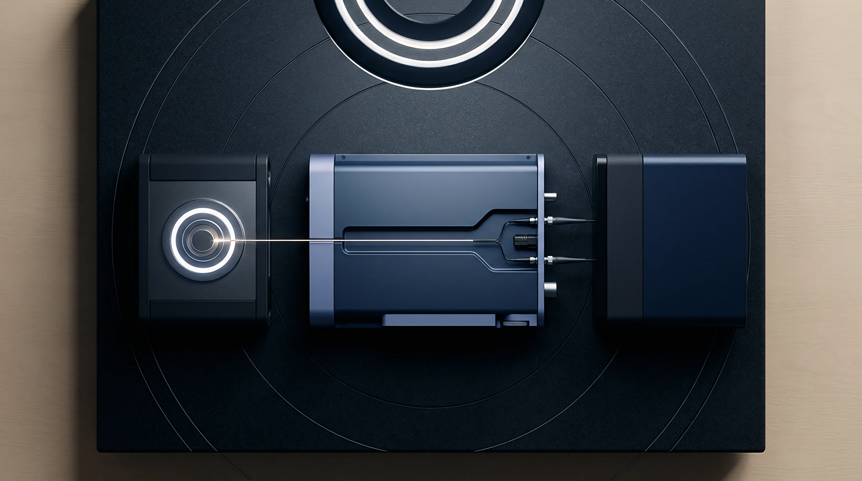
Solid-state drivers generate the current pulses that fire semiconductor laser diodes, while silicon photodiode arrays convert the backscattered light into displacement data. Parasitic inductance along driver traces delays optical emission relative to the master digital clock, which itself drifts with thermal changes. Under pulsed illumination regimes, matching the electronic gate to the optical emission envelope requires direct temporal validation at the optical receiver aperture.
How Do Exposure Delays Corrupt Triangulation Planes?
Coordinate accuracy depends directly on tight synchronization between target illumination and pixel array digitization. Signal propagation through input optocouplers, level shifters, and gate drivers introduces fixed and thermal delays that clip return signals when bandwidth runs tight. If the triangulation sensor scans a continuous surface while the electronic integration period lags behind the illumination trigger, the collected charge centroid drifts along the motion axis.
The calculated height value shifts simply because the sensor samples a point physically downstream from the nominal inspection coordinate.
| Subsystem Element | Nominal Latency Band | Jitter Variance | Spatial Skew at 25 m/s |
|---|---|---|---|
| Laser Diode Current Driver | 3.2 ns to 8.5 ns | ±0.4 ns | 0.08 µm to 0.21 µm |
| CMOS Pixel Global Shutter Gate | 12.0 ns to 28.0 ns | ±1.8 ns | 0.30 µm to 0.70 µm |
| Isolated Sync Inbound Optocoupler | 18.0 ns to 45.0 ns | ±4.5 ns | 0.45 µm to 1.12 µm |
| FPGA Serialization Pipeline | 5.0 ns to 10.0 ns | ±0.2 ns | 0.12 µm to 0.25 µm |
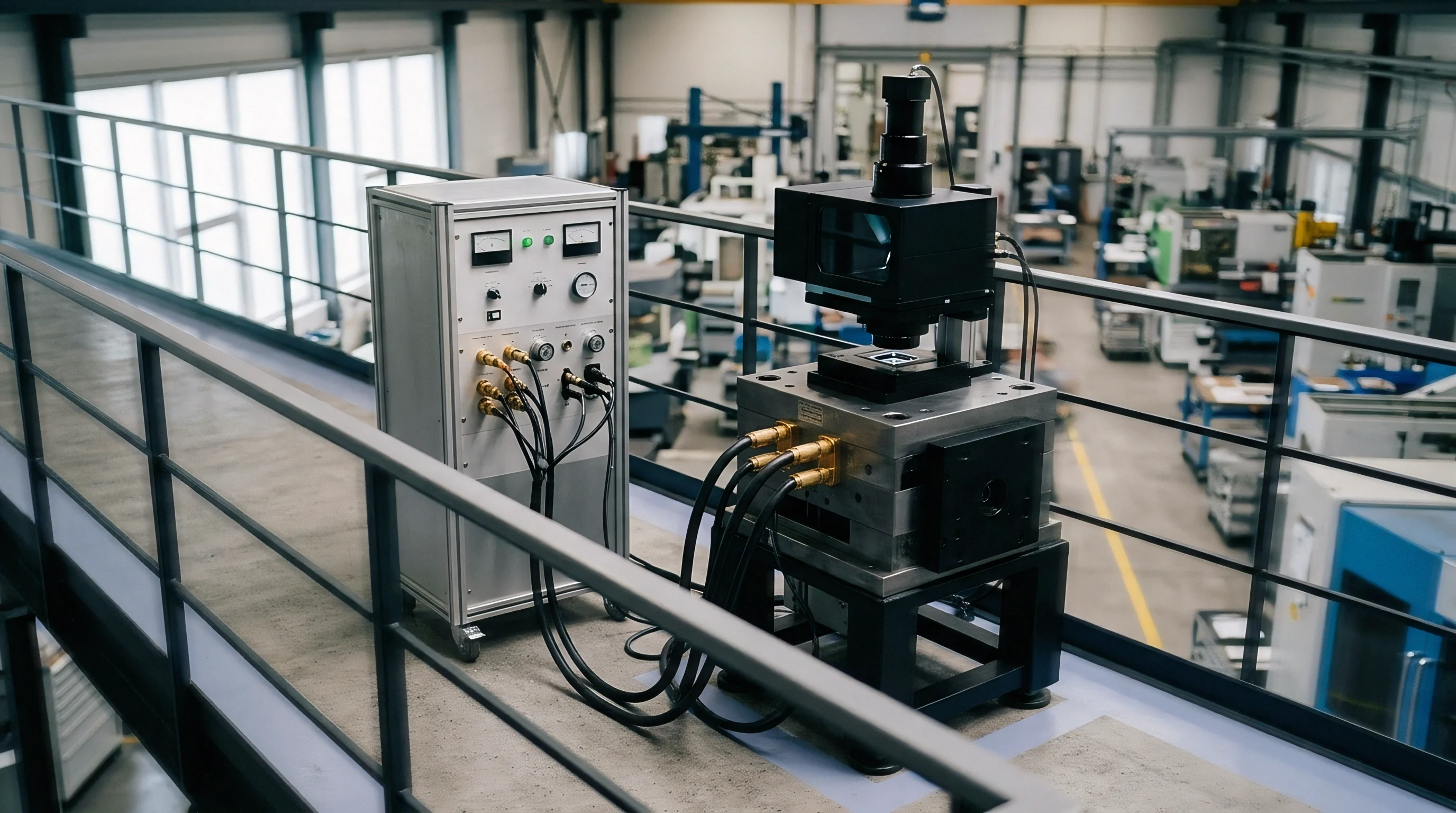
Isolating front-end latency requires probing both the electrical trigger signal and the optical emission envelope with high-bandwidth bench instruments. Tying a picosecond-response optical receiver to a real-time oscilloscope alongside the primary logic trigger exposes internal propagation delays directly. Characterizing this alignment across the expected temperature range establishes the baseline phase tables needed before optical subassemblies are sealed.
Jitter
Phase stability drops rapidly once high-speed sensors interface with external motion hardware. Rotary quadrature encoders, linear scales, and host line-scan controllers route synchronization pulses through long industrial harnesses where propagation delays mount. Across factory floors, electromagnetic interference, ground bounce, and cable capacitance round off sharp square-wave edges, feeding phase-jittered signals into the sensor input terminals.
Internal field-programmable gate arrays process these incoming triggers via phase-locked loops and input deserializers, whose phase locks often slip during abrupt acceleration. Crossing clock domains between the asynchronous trigger input and the internal acquisition engine adds quantization jitter equal to the sensor master clock period. At a sampling rate of one hundred kilohertz, a two-hundred-megahertz master clock introduces five nanoseconds of variable quantization uncertainty, registering false surface height chatter on flat moving parts.
- Asymmetric Pulse Degradation alters the duty cycle of incoming quadrature triggers, causing the interpolation engine to miscalculate instantaneous target velocity and trigger exposures at non-uniform spatial intervals.
- Clock Domain Quantization introduces variable timing offsets between the external encoder capture event and the internal sensor readout frame, generating periodic spatial ripple across digitized profiles.
- Thermal Oscillator Shift causes local clock references to drift against the host system timebase, expanding phase lag during continuous multi-hour production runs.
- Ground Loop Induction injects common-mode electrical noise into single-ended trigger lines, resulting in false trigger events or dropped profile points during high-current motor operations.
Profile reconstruction algorithms assume strictly uniform time intervals between scans. When jitter disrupts that cadence, the spatial frequency spectrum of the calculated surface finish distorts. The firmware locates height by finding the energy centroid on the detector matrix, but high-frequency jitter smears the integrated spot across neighboring pixels, blunting resolution and generating phantom roughness values on mirror-finished stock.
A mechanical reference datum transfers cleanly only when electronic trigger phase tracks physical surface displacement.
Uncalibrated trigger jitter degrades part-sorting accuracy on automated production lines, leading inspection systems to reject good parts or pass out-of-spec dimensions that bind during downstream mechanical assembly.
Target
Physical calibration standards provide the absolute spatial and temporal references required to track phase lag in high-speed triangulation setups. Static optical targets confirm spatial linearity, lens distortion mappings, and focal depth resolution. Measuring dynamic phase lag, however, requires artifacts moving at known, repeatable velocities across the optical axis, translating electronic delays into measurable geometric offsets.
Diamond-turned aluminum wheels and rotating glass-ceramic discs serve as the primary dynamic targets, offering clean knife edges and defined step features. Dynamic test benches spin these discs at rim speeds up to fifty meters per second. While basic shaft encoders can inject significant jitter, dedicated optical encoders mounted right to the air-bearing spindle provide sub-arcsecond angular feedback, separating spindle runout from sensor timing delay.
Contractual compliance under ISO 10360 standards demands documented trigger-to-acquisition latency logs before factory signoff.
Precision Stepped Discs and Calibration Wheels
Machining tolerances on dynamic calibration wheels set the lower bound for phase validation accuracy. Stepped disc teeth undergo coordinate measuring machine inspection to document step heights within sub-micron tolerances before mounting. Alternating reflective and absorbing coatings on the disc surface test how the optical receiver copes with abrupt optical transitions at speed.
Spinning an alternating step past the sensor reveals electrical delay alongside optical settling time. As a step edge sweeps across the beam, the receiver circuitry registers a sharp displacement transition. Any internal phase lag appears as rounding or a lateral shift of the step edge along the motion axis.
Comparing scans collected under forward and reverse rotation isolates this velocity-dependent phase lag from static optical distortion.
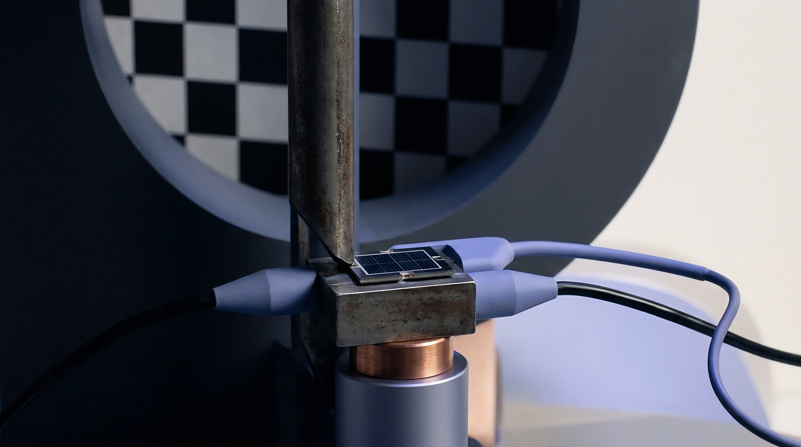
When Do Optical Transfer Jigs Disclose Latency?
Transfer rigs expose internal sensor latency when the peripheral velocity of the test target increases in controlled steps while spatial trigger intervals remain fixed. At crawl speeds, the sensor outputs a profile identical to static calibration data. As surface speed climbs toward production limits, internal phase lag pushes physical features forward along the scan path.
Plotting measured feature position against target velocity yields a linear slope whose gradient equals the total system latency in seconds.
- Mount the optical triangulation sensor onto the rigid three-axis positioning stage of the air-bearing spindle calibration bench.
- Align the sensor optical measurement axis perpendicular to the tangential velocity vector of the stepped calibration wheel to suppress out-of-plane Abbe errors.
- Connect the direct spindle encoder output to the sensor external trigger input using matched fifty-ohm impedance transmission lines.
- Record one thousand revolutions of profile data at a surface speed of one meter per second to establish the static baseline spatial reference.
- Increase spindle velocity in five-meter-per-second increments up to the maximum target speed, capturing identical sample counts at each plateau.
- Compute the spatial cross-correlation between profiles recorded at high speed and the baseline profile to extract net phase lag.
| Detector Architecture | Integration Method | Readout Clock Rate | Dynamic Phase Uncertainty |
|---|---|---|---|
| Standard CMOS Line Array | Rolling Shutter Gate | 40 MHz | ±14.2 ns |
| High-Speed CMOS Line Array | True Global Shutter | 100 MHz | ±2.1 ns |
| Area CMOS in Line Mode | Pipelined Global Shutter | 160 MHz | ±1.4 ns |
| Custom Photodiode Matrix | Direct Parallel Readout | 250 MHz | ±0.6 ns |
Internal DSP routines are often assumed to compensate for motion delays automatically across all operating speeds, yet physical front-end delays still produce dimensional offsets unless low-level hardware timing registers can be adjusted directly.
Wedge
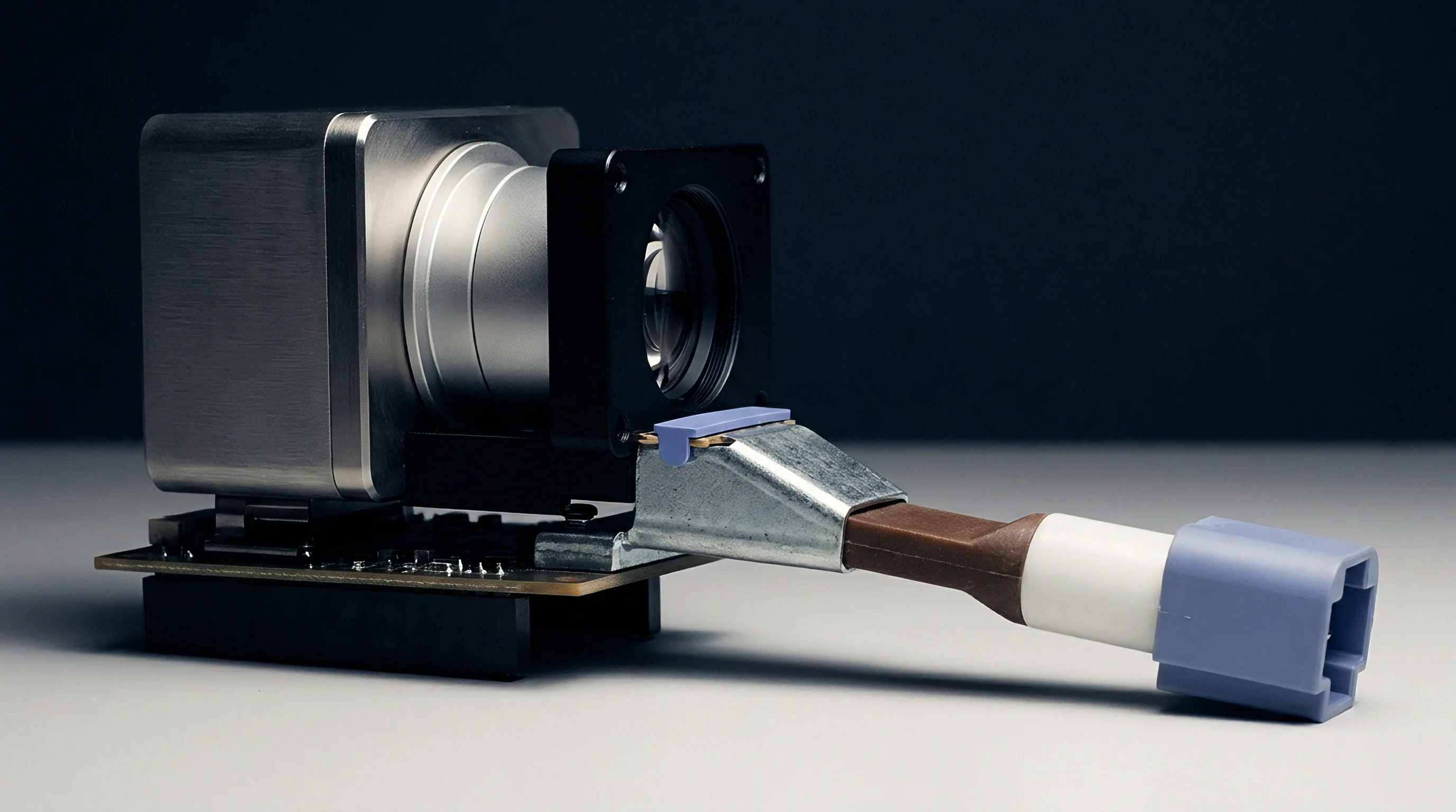
Extracting phase alignment errors mathematically relies on spatial cross-correlation and convolution models. A physical calibration wedge provides a continuous, known slope angle that ties lateral position directly to vertical elevation. When this wedge translates beneath the sensor beam, lateral phase lag registers as an apparent vertical offset, magnifying small temporal errors into obvious geometric steps.
Processing the sensor data requires isolating dynamic phase shifts from static geometric aberrations. Static correction matrices handle lens distortion, Scheimpflug focal tilt, and non-linear pixel spacing, while dynamic errors scale directly with velocity. By pulling the wedge across the beam at an independently verified, constant speed, the total temporal delay emerges through closed-form geometric projection.
Phase Error Transfer Equations and Centroid Convolution
Let an optical triangulation sensor measure an inclined plane with slope tangent alpha. The target translates along the horizontal axis at a constant velocity vector V. The instantaneous true surface height at time t follows the relation H(t) = V t tan(alpha). The sensor electronics introduce an uncompensated system delay tau, comprising optical integration centroid lag, amplifier rise time, and processing pipeline latency.
The sensor samples the surface at discrete nominal trigger intervals T_k. Due to internal delay tau, the captured optical return corresponds to the physical target position at time T_k minus tau. The measured height H_m(T_k) reflects this temporal shift:
H_m(T_k) = V (T_k – tau) tan(alpha)
The apparent spatial error Delta_H between the observed profile and the true physical datum directly yields the system phase delay:
Delta_H = H_true(T_k) – H_m(T_k) = V tau tan(alpha)
Solving for the total system phase delay tau produces:
tau = Delta_H / (V tan(alpha))
This formulation isolates the temporal lag parameter from static sensor scaling constants. When the surface velocity V and the slope angle alpha are verified through independent metrology, the spatial height error Delta_H directly yields the internal phase latency of the optoelectronic system.
A phase mismatch of twelve nanoseconds yields thirty-two micrometers of absolute lateral position error at twenty-five meters per second target velocity.
Worked Triangulation Timing Calculation
To demonstrate the magnitude of this effect in production gauging, evaluate a high-speed line scan optical triangulation sensor operating over a high-velocity steel strip line. Assume the following operational parameters:
The target moves at a velocity V of twenty meters per second. The optical triangulation angle theta sits at thirty degrees. The objective lens system operates with an optical magnification factor M of 0.5.
The sensor uses a high-speed CMOS line array with a pixel pitch P of seven micrometers. The sensor samples profiles at a line rate of one hundred kilohertz, defining a frame interval of ten microseconds. The laser diode current driver exhibits a pulse delay of twelve nanoseconds, while the optocoupler isolation circuit adds twenty-eight nanoseconds of delay.
The internal FPGA signal processing pipeline introduces four clock cycles of latency at an internal clock frequency of one hundred megahertz, contributing forty nanoseconds of digital delay.
Summing these discrete front-end delays defines the raw uncompensated phase lag tau_raw:
tau_raw = 12 ns + 28 ns + 40 ns = 80 ns
During this eighty-nanosecond window, the steel strip moves laterally through a distance Delta_X:
Delta_X = V tau_raw = (20 m/s) (80 10^-9 s) = 1.60 µm
The optical system images this lateral displacement onto the CMOS detector array. Under Scheimpflug geometry with magnification M and triangulation angle theta, the lateral physical shift Delta_X translates into an apparent spot shift Delta_S on the sensor array:
Delta_S = Delta_X M sin(theta) = 1.60 µm 0.5 sin(30°) = 0.40 µm
Expressed as a fraction of the pixel pitch P:
Pixel Shift = 0.40 µm / 7.0 µm = 0.0571 pixels
Modern sub-pixel centroid algorithms achieve nominal interpolation resolutions of one-fiftieth of a pixel (0.02 pixels). An uncompensated phase lag of eighty nanoseconds generates a spot centroid error nearly three times larger than the basic algorithmic interpolation threshold of the instrument. If the surface carries an elevation feature with a slope angle of forty-five degrees (tan(alpha) = 1.0), the vertical height calculation records a direct error Delta_H:
Delta_H = Delta_X tan(alpha) = 1.60 µm 1.0 = 1.60 µm
In precision manufacturing processes where total allowable dimensional tolerances are held within two micrometers, this uncalibrated phase delay consumes eighty percent of the entire product error budget.
Optical Delay Line Alignment Checklist
Implementing reliable phase validation requires structured bench verification criteria before equipment deployment.
- Optical Pulse Alignment confirms that the peak of the laser emission pulse coincides with the center of the detector exposure window within three nanoseconds.
- Trigger Cable Impedance Matching terminates all incoming synchronization lines with characteristic fifty-ohm loads to eliminate signal reflections and false threshold crossings.
- Bidirectional Motion Verification scans the physical calibration wedge in both forward and reverse directions, calculating the spatial divergence between resulting point clouds.
- Thermal Stabilization Soak runs the sensor at full line rate for sixty minutes prior to taking phase validation data to ensure electronic components reach equilibrium operating temperatures.
| Subsystem Stage | Propagation Shift at 20°C | Propagation Shift at 45°C | Propagation Shift at 65°C |
|---|---|---|---|
| Laser Diode Current Driver | 4.1 ns | 5.3 ns | 6.8 ns |
| Optocoupler Input Stage | 22.4 ns | 29.8 ns | 38.2 ns |
| CMOS Pixel Shutter Driver | 14.0 ns | 15.2 ns | 17.1 ns |
| Total Phase Lag Drift | 40.5 ns | 50.3 ns | 62.1 ns |
| Test conditions: ambient chamber cycling, forced convection, baseline measured against primary optical reference receiver. | |||
Whether thermal stabilization algorithms can reliably model and cancel optoelectronic drift without dedicated temperature sensors placed directly adjacent to the photodiode die remains an open question in sensor packaging design.
Remedy
Securing reliable high-speed optical triangulation hardware requires contractual and architectural clarity during procurement. Off-the-shelf turnkey units conceal internal clocking architectures, presenting buyers with sealed modules where phase offsets cannot be inspected or corrected. Semi-custom module agreements must establish unambiguous boundaries regarding register-level firmware access, internal FPGA source code, and factory calibration routines.
Integration contracts divide labor between hardware fabricators and systems integrators. If the sensor supplier locks down low-level DSP timing registers, the integrator cannot insert real-time phase compensation values derived from dynamic wedge calibration. Industrial buyers protect multi-axis programs by negotiating terms that include register maps, clock-tree schematics, and test benches capable of verifying phase latency during incoming inspection.
Deliverable Ownership and Register Access
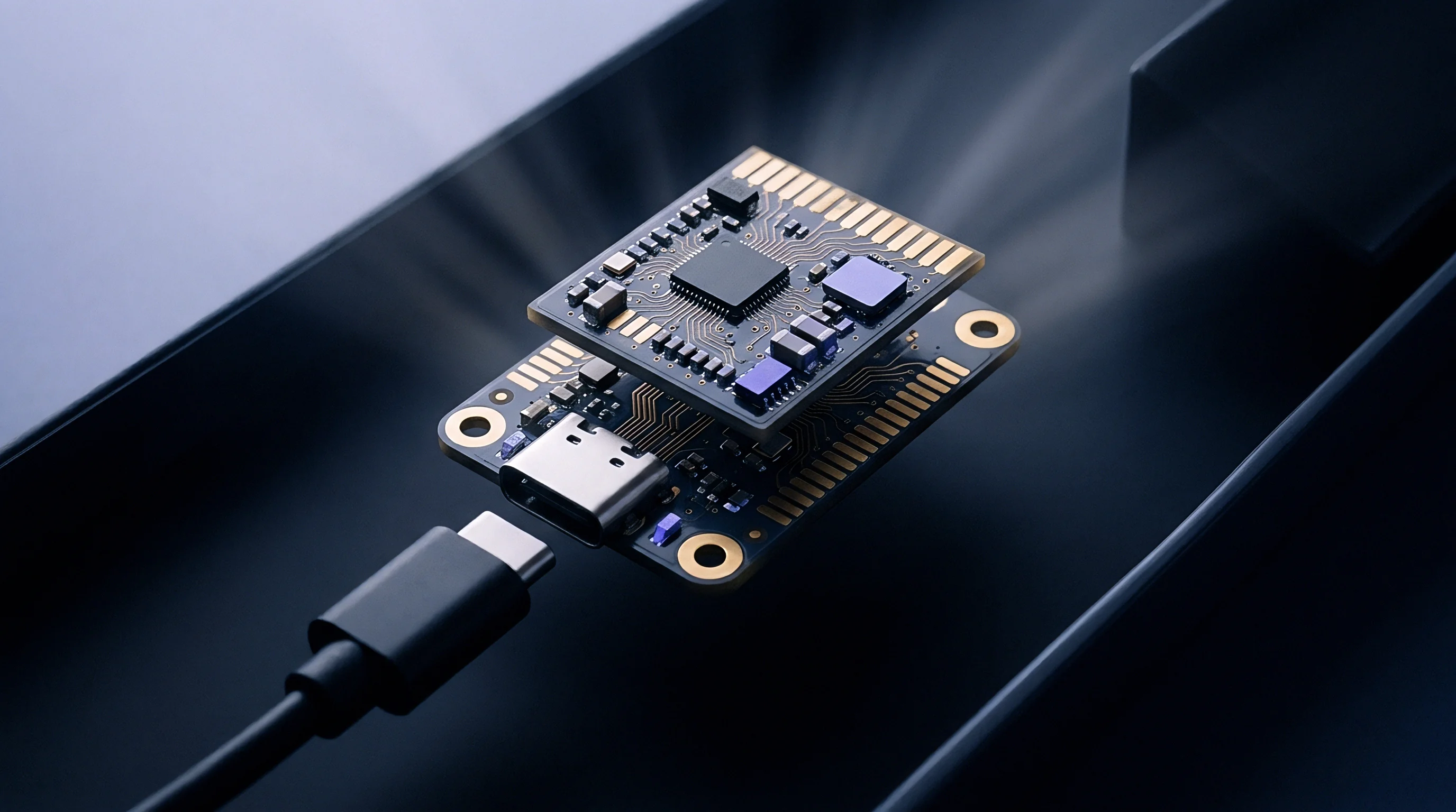
Standard commercial module terms limit customer control to high-level application programming interfaces with proprietary register access keys. Sourcing engineering teams resolve this limitation by specifying custom firmware deliverables in the initial statement of work. Statements of work need to itemize low-level controls, including exposure delay offset registers, trigger input filter clock divisors, and decimation pipeline bypass modes.
Retaining direct register access allows integration engineers to write dynamic phase compensation offsets straight into the FPGA processing pipeline. When dynamic calibration uncovers an eighty-nanosecond propagation lag, the control software writes an offset into the master trigger counter, aligning optical data acquisition with actual part position before profiles reach the factory network.
Dual Sourcing Qualification Safeguards
Qualifying second-source suppliers for optical triangulation heads requires far more than mechanical drawings and parts lists. Variations in passive component tolerances, PCB trace lengths, and optical receiver packaging alter internal propagation delays, creating subtle timing mismatches between supposedly identical hardware revisions.
A functional design transfer package includes dynamic calibration bench drawings, stepped test wheel specifications, and automated cross-correlation test scripts. Factory acceptance test procedures must define enforceable limits for dynamic phase lag across the full operating velocity envelope. Holding alternate suppliers to documented dynamic phase limits prevents the delivery of revision-controlled units that pass static bench checks but drift under dynamic production line conditions.
Uncalibrated hardware latency consumes precision margins before manufacturing begins.