Resolving Low Frequency Field Uniformity Disparities between Compact Pre Scan and Full Certification Facilities
Applying spatial transfer matrices reconciles compact chamber field non-uniformities, eliminating 12 dB pre-scan error margins and preventing retests.

Grid
Testing radiated immunity and emissions between 26 MHz and 200 MHz gets difficult inside compact pre-scan enclosures. The physical dimensions of a three-meter semi-anechoic room or small pre-qualification cell come close to the actual wavelength of low-frequency radio waves. At 30 MHz, free-space wavelength is ten meters ~ well over the internal space of standard pre-scan booths.
Conductive walls, ceiling absorbers, and ground planes reflect energy back into the enclosure, creating standing wave patterns and unstable field levels across the working area.
Full certification labs evaluate radiated immunity under IEC 61000-4-3, which defines a 1.5-by-1.5 meter Uniform Field Area grid set 0.8 meters above the ground plane. To comply, field strength across at least 75 percent of the test points (twelve of sixteen locations) must land within a 0 dB to +6 dB window relative to the nominal field. Accredited ten-meter chambers use deep hybrid ferrite-pyramidal absorbers to achieve high return loss and keep the vertical calibration plane uniform.
Compact pre-scan setups rarely match that environment. Below 100 MHz, smaller test chambers regularly show spatial field swings from -6 dB to +12 dB across that same sixteen-point grid. Testing a device inside a non-uniform pre-scan chamber exposes it to local field spikes or deep nulls that would not occur in a compliant ten-meter room.
That leads either to over-testing and unneeded redesigns, or under-testing that lets non-compliant hardware slip through to final qualification.
These low-frequency standing waves significantly distort field distribution across the test volume.
Calibration Planes and Metrological Definitions
Calibrating the test plane involves placing an isotropic E-field sensor at sixteen grid points arranged in a four-by-four square with 0.5-meter spacing. This run is performed with the turntable empty. As the frequency steps upward ~ usually in 1 percent logarithmic increments from 26 MHz ~ drive power to the transmit antenna increases until the probe hits the target field strength, like 3 V/m or 10 V/m.
Evaluating compact pre-scan enclosures against ten-meter certification facilities shows that forward power recorded to establish target field strength varies drastically per grid point. In a full ten-meter chamber, low-frequency wall reflections remain minimal because of the absorber depth and generous working volume, keeping forward power curves across adjacent points within a tight 2 dB band. In a compact three-meter room, reflections produce interference nodes only fractions of a meter apart, driving power requirements up to 15 dB apart between neighboring points on the plane.
| Frequency Band (MHz) | Pre-Scan Chamber Volume (m³) | Certification Chamber Volume (m³) | Pre-Scan Grid Variance (dB) | Certification Grid Variance (dB) |
|---|---|---|---|---|
| 26 ~ 50 | 45 | 1200 | +11.8 / -5.2 | +3.1 / -0.8 |
| 50 ~ 80 | 45 | 1200 | +9.4 / -4.1 | +2.4 / -0.6 |
| 80 ~ 100 | 45 | 1200 | +7.1 / -3.0 | +1.8 / -0.4 |
| 100 ~ 200 | 45 | 1200 | +4.5 / -2.1 | +1.2 / -0.3 |
Chamber Dimensions and Boundary Interactions
Resonance occurs when enclosure dimensions align with multiples of a wavelength.
Shielded enclosures behave like resonant cavities when their dimensions match multiples of a half-wavelength. A compact pre-scan booth measuring 3 meters wide, 4 meters long, and 2.4 meters high develops basic cavity modes starting around 37.5 MHz. At resonance, field patterns shift sharply with minor changes in position, antenna placement, or cable routing, concentrating fields along modal axes and steepening gradients across the grid.
Absorber layout in smaller chambers worsens the problem. Ferrite tiles rely on magnetic hysteresis to absorb low-frequency fields, but their performance drops off below 30 MHz unless backed by matching foam pyramids. Where tight enclosure dimensions prevent installing deep hybrid absorbers, RF energy bounces off metal walls back into the working volume.
Those reflections distort the wavefront from the biconical or log-periodic transmit antenna, tilting the field plane and ruining phase symmetry.
IEC 61000-4-3 Clause 6.2 allows probe positioning errors of no more than 25-millimeter from specified grid coordinates, which forces labs using compact chambers to build rigid mechanical alignment rigs to keep spatial error under control.
Coupling
Antenna coupling to surrounding enclosure surfaces is another key driver of low-frequency measurement discrepancies. In ten-meter facilities, the transmit antenna sits at least three meters clear of walls and ceiling. In a compact pre-scan setup, elements frequently sit within one meter of ferrite-lined walls, creating strong interaction between the radiator and nearby metal.
That near-field coupling shifts the radiation impedance of biconical and log-periodic antennas at low frequencies. As elements get close to a conductive boundary, reactive energy builds in the space between the elements and wall treatment. This reactive loading alters the VSWR, causing significant input mismatch.
The amplifier then drives a shifting load, varying antenna gain and radiated power across the 26 MHz to 80 MHz sweep.
The metal floor adds more complexity. Semi-anechoic chambers use a conductive ground plane to mimic real operating environments, generating a two-ray interference pattern at the test grid. In a large chamber, the path difference between direct and floor-reflected rays creates predictable, gradual interference shifts.
In compact chambers, shorter ray paths compress those fringes, causing sharp field oscillations as frequency sweeps.
Unwanted boundary reflections contaminate raw sensor measurements.
Antenna Proximity and Input Impedance Shift
Measurements of hybrid ferrite-foam absorber loading demonstrate that reactive coupling between biconical antenna tips and wall absorbers shifted the measured input reflection coefficient by up to 4.2 dB at 35 MHz. Calibration routines assume a fixed antenna factor throughout the chamber. When reactive loading shifts antenna impedance, published free-space antenna factors no longer accurately map forward power to actual field strength.
This shift disrupts power allocation during calibration runs. To reach a target 10 V/m field strength at an affected grid point, automated software ramps up RF drive to offset near-field coupling losses. That higher drive over-powers adjacent grid points that lack the same loading, widening spatial field variations and creating artificial hotspots.
Absorber performance degrades rapidly when physical cone depth falls below one quarter of the operational wavelength.
Absorber Return Loss at Low Frequencies
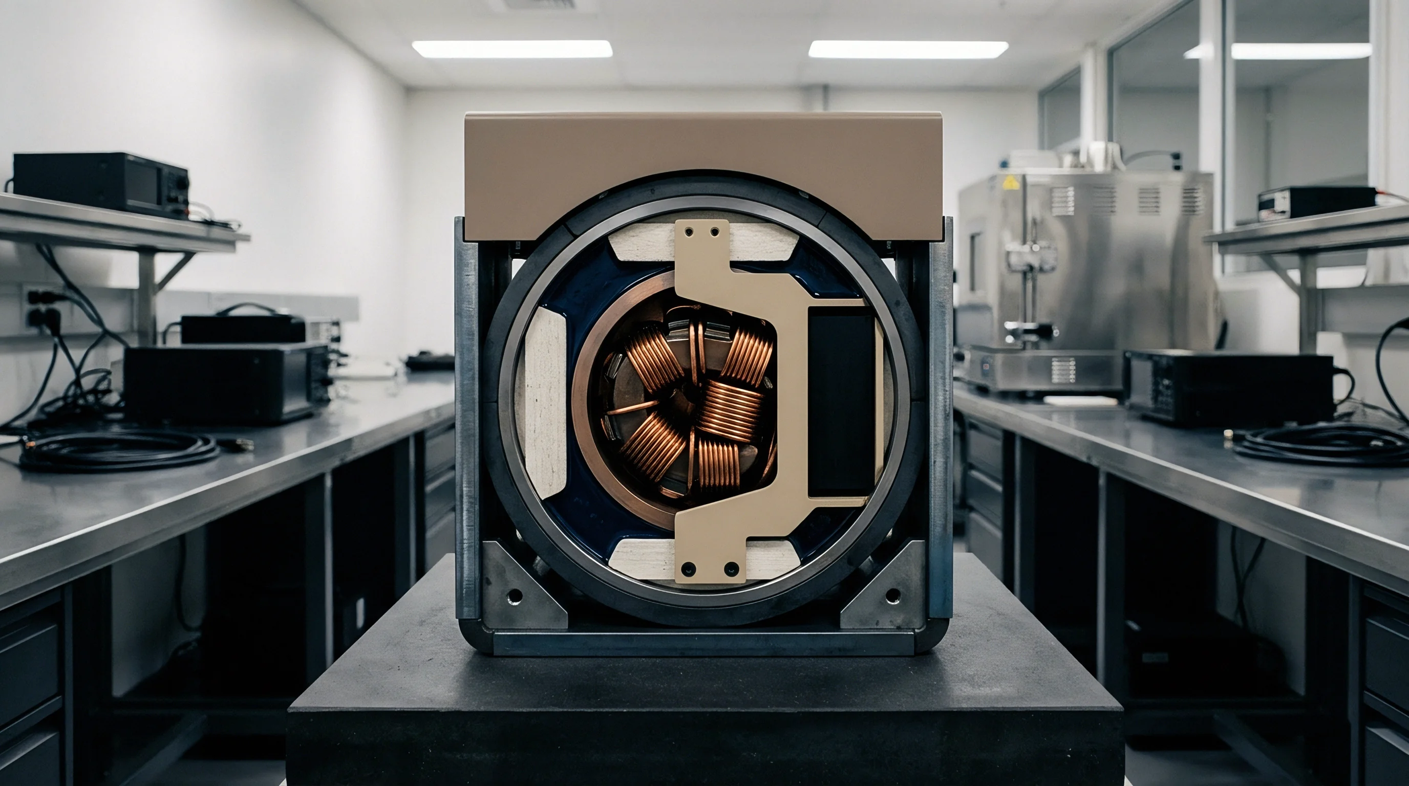
Absorber selection governs how field energy decays inside an enclosure. Ferrite tiles offer a thin profile, but performance hinges on installation quality, panel grounding, and magnetic permeability. Above 100 MHz, ferrite efficiency drops unless paired with carbon-loaded foam pyramids.
Compact rooms frequently compromise on pyramid height to save working space, fitting 30-centimeter or 45-centimeter cones instead of the 1-meter absorbers used in full certification rooms.
Short foam pyramids deliver poor return loss below 80 MHz. At 30 MHz, a 30-centimeter absorber gives less than 3 dB return loss, sending more than 50 percent of incident wave energy straight back into the room. These reflections combine vectorially with the primary wave from the antenna, setting up spatial standing waves across the test volume.
- Ferrite Loading Density specifies the mass of sintered ferrite tiles mounted per square meter of wall area, setting magnetic absorption limits below 50 MHz.
- Absorber Cone Depth defines the geometric impedance matching layer between free space and backplate absorbers, dictating high-frequency transition points.
- Antenna Separation Distance sets the clearance between radiating elements and enclosure walls to prevent reactive near-field loading.
- Ground Plane Boundary Cavities create parasitic inductance loops when metal floor tiles lack continuous electrical bonding at chamber seams.
Field uniformity in compact rooms improves noticeably when engineers observe separation distances calculated for near-field boundaries.
Harmonics
Amplifier non-linearity is a major, frequently overlooked source of field uniformity errors. Producing high field levels like 10 V/m or 30 V/m between 26 MHz and 100 MHz takes significant power because antennas are inefficient at these frequencies. A biconical antenna around 30 MHz typically has an antenna factor between 12 and 18 dB/m, requiring 50 to 200 Watts of RF drive to generate standard field levels at 3 meters.
Driven near their upper output limit, broadband solid-state amplifiers generate harmonic distortion. At a fundamental setting of 30 MHz, an overdriven amplifier produces harmonics at 60 MHz, 90 MHz, and higher multiples. Wideband isotropic probes lack frequency discrimination, measuring the root-sum-square total of all field components across their entire band (often 10 kHz to 6 GHz).
Unfiltered harmonic emissions introduce significant measurement error at the probe.
Power Amplifier Non-Linearity and Probe Response
When an amplifier outputs harmonic content, the isotropic probe measures the combined field of the fundamental and all harmonics. If a 60 MHz harmonic is only 10 dB below the 30 MHz fundamental, the reported field reading runs roughly 0.4 dB above the actual fundamental field strength. If harmonic level reaches 4 dB below fundamental, that error climbs past 1.6 dB.
During automated field calibration, control software adjusts drive power against probe feedback. When harmonic energy artificially inflates probe readings, the software stops ramping generator power early, leaving the actual fundamental field below test requirements. When the Equipment Under Test is subsequently tested, its narrow-band internal circuits respond only to the fundamental, resulting in an under-test condition even though calibration logs show full target field strength.
A second-harmonic level 15 dB below the fundamental frequency introduces a 1.4 dB overestimation error in broad-band isotropic electric field probe readings during field uniformity calibration.

Filtering Strategies and Harmonic Rejection
Certification labs avoid harmonic errors by placing high-power low-pass filter banks between amplifier outputs and transmit antennas. These filter banks switch automatically across the sweep, keeping harmonics at least 20 dB to 30 dB below the fundamental. Pre-scan rooms often omit filter banks to keep costs down, running raw amplifier output straight to the antenna.
- Connect a high-power directional coupler between the amplifier output terminal and the transmit antenna feed cable.
- Route the coupled port of the directional coupler to a calibrated spectrum analyzer fitted with proper input attenuation.
- Run a frequency sweep from 26 MHz to 200 MHz at forward power levels required to generate target field strength.
- Measure fundamental and harmonic power across the sweep to highlight regions where harmonic rejection drops below 20 dBc.
- Insert switchable low-pass filter banks into the RF signal path to suppress harmonic content before it reaches the antenna.
Chamber manufacturers often claim broadband isotropic probes provide accurate total field readings without filtering because probe frequency response remains flat across calibrated ranges.
Correction
Resolving low-frequency field disparities between compact pre-scan rooms and full certification chambers requires systematic calibration transfer matrices. Relying on raw pre-scan data forces engineers to pad margins, often driving target field levels up by 6 dB to 10 dB just to ensure passing at external labs. This over-testing places unnecessary stress on circuitry, prompting unneeded shielding additions and higher bill-of-materials costs.
A spatial transfer matrix H(f) maps local pre-scan field values to the field distribution of a compliant ten-meter facility. This requires characterizing both enclosures with matching isotropic field probes, transmit antennas, and grid geometries. Measuring matrix elements across narrow frequency steps builds a calibration vector that translates pre-scan power settings into normalized field intensities mirroring full-scale chamber behavior.
Harmonic distortion alters the power required across the grid.
Transfer Function Derivation and Virtual Mapping
Deriving an accurate transfer matrix begins by measuring the complex field vector across all sixteen grid points in both the compact pre-scan room (Epre) and the reference ten-meter certification chamber (Ecert). Mapping spatial field deviations across sixteen grid points yields complex transfer coefficients, establishing that matrix correction reduces pre-scan field prediction uncertainty from 7.2 dB down to 1.1 dB across the critical 30 MHz to 80 MHz frequency range. The spatial transfer matrix Hij(f) scales the local pre-scan field vector to match certification chamber performance through linear transformation equations:
Ecert(f) = Hij(f) · Epre(f)
This virtual grid transformation offsets persistent structural non-uniformities caused by cavity modes and wall coupling. Instead of applying uniform drive power based on a single compromised grid location, the control software applies point-specific drive profiles from the transfer matrix, keeping artificial field spikes from distorting overall chamber tolerance calculations.
| Correction Method | 26-50 MHz Error (dB) | 50-100 MHz Error (dB) | 100-200 MHz Error (dB) | Processing Overhead (Min) |
|---|---|---|---|---|
| Uncorrected Raw Pre-Scan | ± 8.5 | ± 6.2 | ± 3.8 | 0 |
| Single-Point Normalization | ± 5.4 | ± 4.1 | ± 2.5 | 2 |
| 16-Point Spatial Transfer Matrix | ± 1.2 | ± 0.9 | ± 0.6 | 15 |
| Virtual Grid Interpolation | ± 0.8 | ± 0.6 | ± 0.4 | 45 |
Spatial Averaging and Matrix Transformation
Spatial non-uniformity across the grid directly alters test margin calculations.
Spatial averaging algorithms refine raw grid data through localized spatial weighting factors. In compact enclosures where field gradients shift over short distances, standard arithmetic averaging across sixteen points masks localized spikes. Weighted spatial averaging applies correlation matrices to smooth resonant peaks while preserving energy conservation across the calibration plane.
Digital pre-distortion algorithms apply these calculated transfer weights directly to signal generator drive levels during immunity pre-scans. The control software checks the current frequency step, queries the transfer matrix, and adjusts generator output amplitude in real time. This ensures the Equipment Under Test experiences a field exposure profile equivalent to a ten-meter chamber, closing the gap between internal pre-scans and external lab results.
EN 61000-4-3 Clause 6.2 invalidates field uniformity calibrations where more than 4 of the 16 grid points exceed the 6 dB window.
Using uncorrected pre-scan drive profiles on sensitive assemblies leads engineering teams to add unnecessary metal shielding and extra line filtering, adding up to $4.50 per unit in avoidable material costs across high-volume production runs.
Validation
Validating mathematical correction models requires structured comparison tests using standardized reference units. A thorough validation checks both immunity thresholds and radiated emissions across compact setups and accredited ten-meter chambers. Testing real-world hardware in both settings confirms whether spatial transfer matrices eliminate false failures and missed passes at low frequencies.
Take a practical trial with a commercial industrial controller evaluated for radiated immunity under EN 61000-4-3 standards (80 MHz to 1000 MHz, 10 V/m target field intensity), extended down to 26 MHz for pre-qualification. The pre-scan chamber has a 3.5-meter by 3-meter floor lined with hybrid ferrite tiles and 30-centimeter foam pyramids, while the certification site uses an accredited 10-meter semi-anechoic chamber. Raw pre-scan sweeps without matrix correction showed five separate immunity failure points between 30 MHz and 65 MHz where microcontroller communication dropped.
Follow-up testing in the accredited 10-meter chamber revealed that four of those five failures were false positives caused by field hotspots in the compact enclosure, where standing waves delivered local field strengths over 22 V/m despite software requesting 10 V/m. Applying a 16-point spatial transfer matrix to the pre-scan routine corrected the drive power levels, clearing all four false failures while correctly isolating the single real vulnerability at 42 MHz.
Measurement uncertainty increases substantially at lower frequencies.
Comparative Laboratory Measurement Correlation
Correlating test results across facilities requires establishing matrix-based transfer functions.
Correlating test setups requires complete uncertainty budgets for both pre-scan and certification environments. Total expanded uncertainty for an accredited ten-meter room during radiated immunity testing typically sits between 1.8 dB and 2.2 dB at a 95 percent confidence level (k=2). Uncorrected compact pre-scan chambers exhibit expanded uncertainties between 5.8 dB and 8.4 dB from 26 MHz to 80 MHz, making raw data too uncertain for compliance decisions.
Applying spatial transfer matrix corrections drops compact chamber expanded uncertainty down to 2.6 dB, bringing pre-scan data into reasonable alignment with accredited facility results. This allows engineering teams to make design decisions using internal test results, cutting out redundant external chamber sessions and keeping project schedules on track.
| Uncertainty Contributor | Compact Chamber Uncorrected (dB) | Compact Chamber Corrected (dB) | 10m Certification Chamber (dB) |
|---|---|---|---|
| Field Probe Isotropic Response | 0.80 | 0.80 | 0.50 |
| Amplifier Harmonics / Non-Linearity | 1.50 | 0.30 | 0.20 |
| Spatial Non-Uniformity / Reflections | 4.20 | 0.90 | 0.60 |
| Antenna Distance & Alignment Error | 0.60 | 0.40 | 0.20 |
| Cable Loss & Mismatch Uncertainty | 0.50 | 0.30 | 0.20 |
| Expanded Uncertainty (k=2) | 9.32 | 2.74 | 1.71 |
Financial and Lead Time Risk Matrix
Relying on uncorrected pre-scan data carries real financial risk during qualification cycles. Failing a formal test at an accredited lab introduces typical delays of four to six weeks for root-cause analysis, redesign work, prototype builds, and re-booking chamber time. With accredited lab rates running $2000 to $3500 per eight-hour test day, repeated failures add up quickly across product lines.
By contrast, mathematical pre-scan alignment requires an initial investment of about 16 calibration hours to characterize the chamber and derive the software matrix. Once generated, the transfer matrix remains valid for up to twelve months as long as chamber layout, antenna mounting, and cabling remain unchanged. Internal pre-scan accuracy improves dramatically, dropping final external test failure rates from 35 percent to under 3 percent across multiple product families.
Can automated AI-driven finite-element field modeling dynamically predict real-time spatial transfer matrices for changing EUT dimensions inside compact chambers without requiring manual 16-point physical grid re-calibrations?