Time Averaged Radiation Assessment for Multi-Transmitter Dynamic Power Backoff in Dense Arrays
Dynamic backoff algorithms optimize dense array power outputs using sliding time windows to maintain maximum throughput within time-averaged exposure limits.


Grid
Modern handheld devices pack dense RF arrays into tight quarters, forcing transceivers right next to each other. When a sub-6 GHz 5G NR module, a Wi-Fi 7 6 GHz array, and a millimeter-wave phased array all run at once inside a space under one hundred cubic centimeters, spatial isolation breaks down. Near-field power distributions turn into intricate coupling networks between elements.
As a result, localized Specific Absorption Rate (in watts per kilogram) strays far from the simple sum of individual conducted power limits, forming dynamic thermal hotspots where fields constructively interfere inside dielectric tissue models.
Static power backoff keeps RF exposure within limits only by crippling system throughput. Older compliance approaches simply slapped a fixed power ceiling on every active transmit path whenever multi-radio operation was triggered. In a triple-active setup, that static backoff could hit six decibels per channel ~ wasting link margin even if actual duty cycles were negligible.
Dynamic backoff algorithms avoid this hit by continually balancing time-averaged exposure across active elements. Transmit state machines log energy over sliding windows, converting rigid peak power limits into flexible temporal budgets.
Inside a millimeter-wave array, spatial power density shifts continuously as beamforming codebooks update every few milliseconds to follow signal reflections. Assessing these radiated fields requires tracking complex vector spatial matrices across every phase state. When several elements fire at once, near-field phase alignment alters reactive energy storage around the enclosure, meaning any compliance framework has to account for both conductive thermal accumulation in tissue and spatial power flux density across high-frequency boundaries.
At a spatial separation of three millimeters from the phantom shell, constructive near-field superposition increases localized spatial peak SAR by 3.2 dB relative to isolated transmitter baselines.

Spatial Interaction in Compact Antenna Structures
Antenna elements spaced less than a wavelength apart interact through mutual impedance and shared ground plane currents. Driving current into one element excites parasitic currents in its neighbors, warping the radiated beam pattern and degrading near-field spatial isolation. This makes the overall power distribution sensitive to immediate environment changes, including how a user holds the device or where metallic structural frames are placed.
Evaluating multi-antenna spatial interaction requires measuring scattering parameters alongside surface field sweeps. Dual-band Wi-Fi designs at 2.4 GHz and 5 GHz tend to launch surface waves along shared ground planes, creating parasitic interference spots near chassis corners. Above 24 GHz, dielectric substrate losses and line leakage distort the near-field pattern even further.
Consequently, test protocols must map peak absorption across a three-dimensional volume instead of relying on single-element orthogonality assumptions.
Evaluating spatial interaction involves analyzing multiple concurrent hazard factors across distinct spatial structures:
- Spatial Mutual Coupling alters current distribution across neighboring radiators, shifting peak spatial absorption regions unpredictable distances from the primary radiator axis.
- Ground Plane Return Currents merge across adjacent transmitter ICs, raising low-frequency field levels near non-radiating conductive enclosures.
- Dielectric Detuning induced by tissue proximity alters antenna input impedance, driving reflection coefficient changes that shift power amplifier loading.
- Constructive Field Superposition multiplies peak power density wherever phase-aligned fields cross within high-permittivity phantom tissue.

Thermal Constraints and Transceiver Coupling Modes
Human tissue absorbs RF energy through ionic conduction and dielectric relaxation, converting field energy directly into thermal rise. International standards set maximum time-averaged absorption limits to keep tissue heating under one degree Celsius. Because modern dense arrays operate right near these limits, dynamic thermal management is essential.
Tracking localized surface heating under unmitigated dynamic array conditions shows up to 1.8 dB of spatial deviation. Power amplifiers running at high duty cycles heat up at the junction, shifting output stage impedance matching. That thermal drift alters radiated power and throws off pre-calibrated backoff tables.
To compensate, control logic combines temperature sensor feeds with transmit timing logs so the array stays predictable during sustained high-power bursts.
Assessing dynamic behavior requires constantly weighing thermal drift against spatial coupling matrices. If a device pulls down a large file over multi-carrier cellular while hosting a Wi-Fi hotspot, the power amplifiers heat up localized regions of the board. That heat alters substrate dielectric constants, shifting antenna tuning and near-field radiation.
Compliance models have to evaluate these feedback loops in real time so heavy processing spikes do not trigger transient exposure violations.
How does spatial power distribution behave when dynamic phase shifts alter element phase relationships in real time? This question keeps assessment practices evolving as engineers work to capture worst-case spatial SAR trajectories.
Algorithm
Dynamic backoff logic relies on continuous energy budget calculations over sliding time windows. Standard regulations specify exposure limits over intervals between ten and six hundred seconds, depending on the frequency band and body exposure rules. The central backoff software logs instantaneous power values into a circular buffer at millisecond intervals, integrating delivered power over time to project exposure trends and pull back transmit power before crossing legal thresholds.
When an active link demands peak power for high-throughput bursts, the algorithm allows temporary excursions above the continuous exposure baseline. Once total energy in the sliding window nears the regulatory cap, the state machine steps down conducted power across active chains. Managing power headroom this way protects link budgets during initial connection setup while guaranteeing compliance over the full averaging window.
Sliding Window Mechanics and Energy Budget Tracking
Sliding window algorithms split exposure accounting into standardized time frames. Under FCC rules, sub-6 GHz absorption is typically evaluated over 100 seconds, compared to 60 seconds under European norms. Millimeter-wave signals use shorter windows ~ 10 to 30 seconds ~ because higher frequencies produce rapid surface heating.
Across all active transmitters, the algorithm sums normalized exposure contributions simultaneously to keep total normalized SAR below unity.
The energy tracking algorithm calculates total exposure using a normalized summation across active frequency bands and antenna elements:
This summation updates continuously. When cumulative exposure reaches a soft threshold ~ usually set around 85 percent of the maximum limit ~ the backoff state machine calculates the necessary drop for each band. It evaluates channel quality, modulation scheme demands, and link priority, cutting power on secondary radios first to protect critical connections.
The table below summarizes standard time-averaging window requirements and power backoff operational parameters across major regulatory domains:
| Regulatory Jurisdiction | Frequency Band Range | Sliding Window Duration | Peak to Average Power Ratio | Backoff Latency Floor |
|---|---|---|---|---|
| United States (FCC) | Sub-3 GHz Cellular / Wi-Fi | 100 Seconds | 3.0 dB | 2.5 Milliseconds |
| United States (FCC) | 3 GHz to 6 GHz Unlicensed | 60 Seconds | 4.5 dB | 2.5 Milliseconds |
| United States (FCC) | 24 GHz to 42 GHz mmWave | 4 Seconds to 10 Seconds | 6.0 dB | 1.0 Millisecond |
| European Union (CE RED) | Sub-6 GHz Multi-Radio | 60 Seconds | 3.0 dB | 10.0 Milliseconds |
| European Union (CE RED) | 24 GHz to 60 GHz mmWave | 120 Seconds (Averaged) | 5.0 dB | 5.0 Milliseconds |
| Japan (MIC / Giteki) | Sub-6 GHz Cellular | 360 Seconds | 2.5 dB | 10.0 Milliseconds |

State Machine Transitions across Multi-Band Arrays
The backoff controller’s transition logic manages complex radio priority rules. If a user starts a voice call on a low-frequency cellular band while streaming data over high-frequency Wi-Fi, the state machine prioritizes the voice budget. It trims Wi-Fi power quickly to make headroom for cellular transmission, deriving decay rates directly from historical energy levels in the sliding window buffer.
The regulatory evaluation procedure for time-averaged backoff algorithms demands structured compliance validation:
- Connect conducted RF test ports of all active transmitters to high-speed power sensors synchronized with a base station emulator.
- Initialize radio links at baseline power levels to establish stable sliding window buffer states across all operational bands.
- Inject a maximum power transmission request on Channel A while maintaining active background transmission on Channel B.
- Log continuous power levels at sample intervals non-exceeding five milliseconds across the full duration of the standard time window.
- Verify that calculated cumulative normalized exposure remains strictly under unity throughout transient state steps.
- Trigger a simulated path loss event forcing handoff to maximum power on Channel B and observe dynamic backoff step performance on Channel A.
- Download internal firmware time-stamped log files and cross-examine internal algorithm state decisions against external power sensor recordings.
Firmware lookup tables map instantaneous power to exposure coefficients, which requires careful factory calibration across temperature ranges and component tolerances. Beam steering adds another layer of complexity in millimeter-wave systems, as spatial power density shifts with every codebook index. To maintain accurate exposure tracking, the state machine checks active beam indices alongside conducted power metrics.
A properly calibrated dynamic backoff mechanism restores full transmit power as soon as older energy samples drop out of the sliding window buffer, keeping the link budget as high as possible.

Chamber
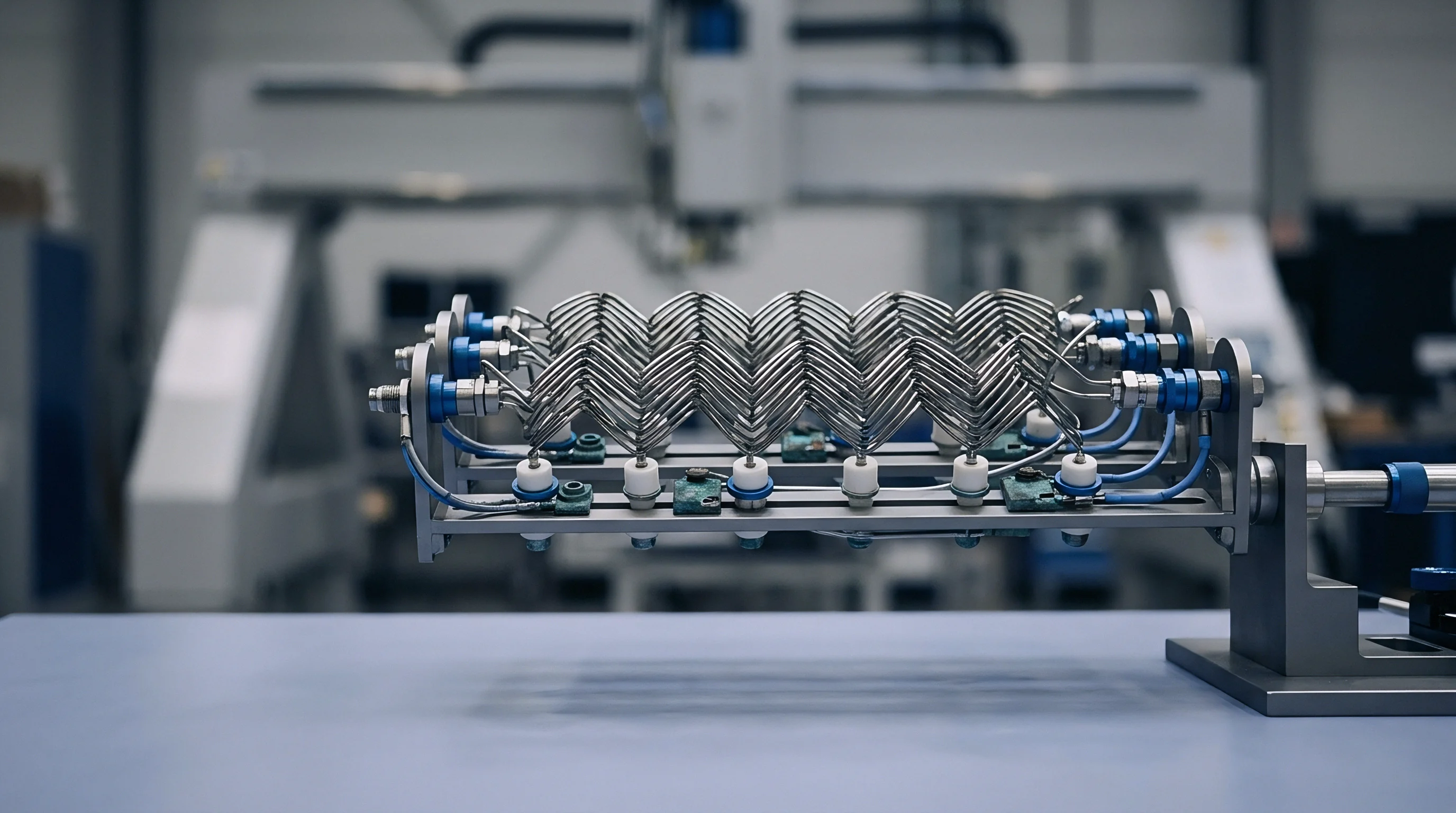
Validating time-averaged backoff behavior requires test chambers equipped with fast vector measurement gear. Traditional single-probe robotic SAR scanners take up to forty minutes to finish a full 3D volumetric scan over a phantom shell ~ far too slow for transceivers shifting power states every few milliseconds. Instead, test labs use multi-probe arrays and vector E-field reconstruction chambers to capture transient absorption profiles almost instantly.
Probe array systems position multi-axis E-field sensors along an anatomical phantom arch to measure magnitude and phase simultaneously across the exposure surface. By computing full spatial peak SAR in milliseconds, these setups allow labs to record changing power distributions while the dynamic backoff algorithm adjusts active array elements.
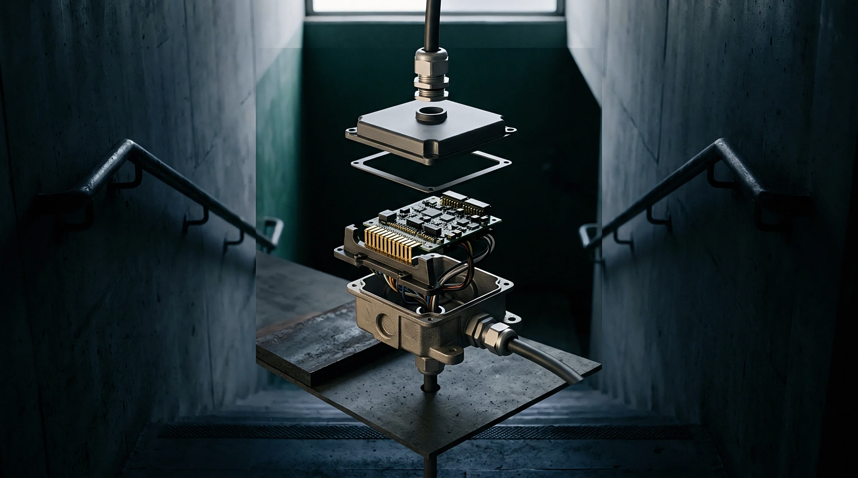
How Does Spatial Scanning Speed Affect Dynamic Compliance Validation?
Robotic probe movement limits measurement fidelity when tracking time-varying signals. If a transmitter drops power by 4 dB halfway through a 30-minute raster scan, the resulting field map is distorted and mathematically invalid. Fast probe arrays avoid physical movement delays by electronically sampling hundreds of fixed sensors built into liquid phantom structures.
Missing backoff timing data in vendor test plans consistently causes chamber delays. Test engineers must synchronize vector probe arrays with time-correlated conducted power logs. While base station emulators issue dynamic power commands to the device under test, high-speed sampling systems capture continuous antenna port power vectors, tying internal software logs to external radiated field measurements.
IEC IEEE 62209-1528 mandates that time-averaged exposure measurement systems maintain a temporal measurement sampling rate fast enough to track instantaneous power state changes without aliasing transient overshoot events.
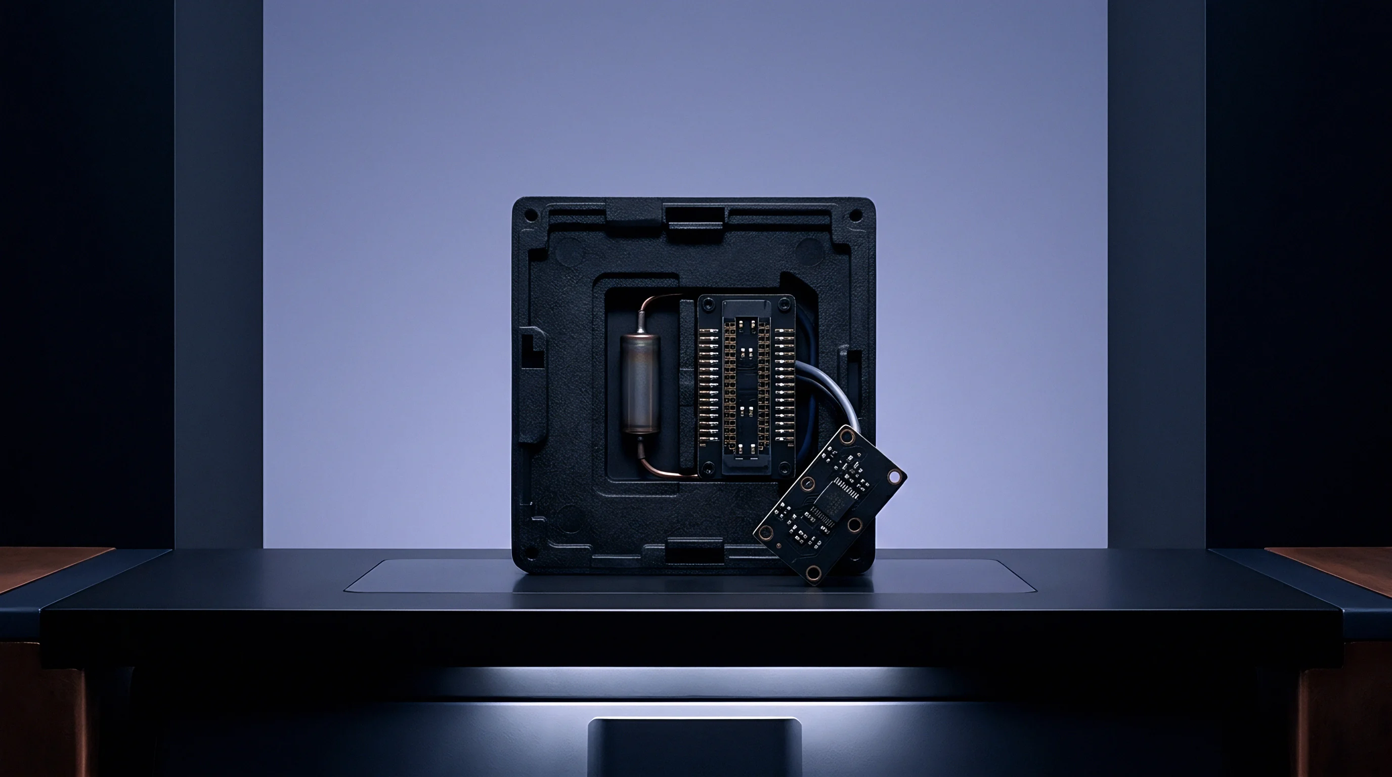
Vector Probe Arrays and Transmit Sequence Triggering
Chamber calibration accounts for physical coupling between probe arrays and the device housing. Using calibration matrices derived from standard dipole sources, these systems reconstruct unperturbed spatial fields. Sensor arrays embedded in flat and head phantoms capture complex electric field vectors, letting processing software generate volumetric SAR maps in real time.
Testing millimeter-wave dynamic backoff requires free-space power density setups with calibrated planar or spherical probe arrays placed in the near-field region. Phase-retrieval algorithms then compute spatial power density across evaluation planes positioned five millimeters off the device housing.
Hardware triggering synchronizes data capture across all channels. Base station emulators send continuous power control commands over RF or direct lines, driving the device between maximum burst states and backoff modes. The probe system captures spatial power profiles at frame boundaries to verify that averaging loops stay within tolerance bounds.
Failing to align probe field data with internal power logs can trigger false regulatory failures, causing unnecessary redesigns and launch delays.


Filing
Securing market access for devices using dynamic backoff requires thorough documentation of algorithm performance and safety margins. Regulatory agencies review dynamic power management closely. Applications sent to the FCC in the United States, notified bodies in the European Union, or regional regulators like SRRC in China must include test reports demonstrating that time-averaged exposure stays below legal limits under all operating conditions.
Filing strategies depend on whether the backoff software runs as a self-contained embedded module or relies on host processor triggers. Modular grant holders have to spell out interface constraints, timing controls, and mandatory antenna layouts in their integration manuals. Meanwhile, host manufacturers integrating pre-certified modules remain legally responsible for verifying host-level field interactions and submitting any necessary permissive change filings.

Regulatory Authorization Paths across Global Markets
Authorization routes vary significantly by region. The FCC requires filings under KDB 447498 D04 alongside specialized KDB inquiries for time-averaged SAR approvals. Submissions must detail software architecture, circular buffer mechanics, control loop response latencies, and lookup table generation, backed by test reports showing real-time power tracking alongside calculated exposure curves.
In Europe, Radio Equipment Directive (2014/53/EU) compliance relies on standards EN 50385 and EN 62209-1528. Regulatory bodies focus on technical documentation proving compliance under worst-case operating modes, requiring clear declarations of thermal algorithm parameters and numerical simulation data validated against chamber measurements.
Preparation of regulatory filing dossiers requires systematic assembly of administrative, technical, and measurement deliverables:
- Algorithm Software Operational Description detailing timing windows, state decision trees, and circular buffer structure signed by lead system engineers.
- Factory Calibration Verification Procedures proving that look-up table backoff offsets are permanently written into secure non-volatile device memory during production line testing.
- Conducted and Radiated Time-Averaged Test Reports containing synchronized temporal power plots and spatial field reconstruction maps generated by accredited laboratory chambers.
- Numerical SAR Simulation Validation Files matching CAD physical models against phantom tissue field distributions under multi-transmitter driving conditions.
- Modular Integration Instructions mandating exact mechanical layout boundaries, spatial separation distances, and thermal dissipation paths for third-party host integrators.

Host Integration Obligations and Permissive Change Thresholds
Updating an existing product line to add dynamic backoff triggers strict re-certification rules. Under FCC guidance, introducing dynamic power management software to a certified module requires a Class II Permissive Change. Manufacturers must submit test data proving the modified firmware does not create unverified operational states or push peak spatial exposure past original grant limits.
The table below compares primary regulatory filing attributes, test requirements, and administrative documentation demands across key global market destinations:
| Market Jurisdiction | Primary Standard Framework | Filing Approval Route | Mandatory In-Country Physical Testing | Permissive Change Process Class |
|---|---|---|---|---|
| United States | FCC Part 2 / KDB 447498 D04 | TCB Grant via KDB Inquiry | No (Accredited Lab Data Accepted) | Class II Permissive Change (C2PC) |
| European Union | CE RED / EN 62209-1528 | EU Type Examination Certificate | No (CE DoC with Notified Body) | Technical Construction File Update |
| Canada | ISED RSS-102 / SPR-004 | TAC Certificate via FCB | No (Accredited Lab Data Accepted) | Category IV Permissive Change |
| China | SRRC Decree 15 / GB 21288 | SRRC Type Approval Certificate | Yes (State Accredited Lab Testing) | Full Re-certification File Submission |
| Japan | MIC Ordinance 37 / Giteki | Registered Certification Body | Optional (Local Agency Verification) | Modification Filing to Existing Grant |
| Brazil | ANATEL Act 1630 / Act 7280 | ANATEL Homologation Certificate | Yes (In-Country Local Lab Testing) | Certificate Maintenance Update |
Modifying dynamic backoff timing parameters or expanding look-up table backoff steps in device firmware invalidates existing SAR compliance reports, triggering mandatory Class II Permissive Change filings across all active market approvals.
Integration documentation must explicitly prohibit third-party software from altering or overwriting calibrated power management tables stored in non-volatile memory. Regulatory auditors regularly inspect device security to ensure custom firmware or root access cannot bypass exposure controls.
Under FCC Part 2.1043, any modification to power control algorithms that alters output duty cycles beyond grant tolerances requires updated test reports and revised operational descriptions before commercial distribution.


Invoice
Compliance testing costs for dynamic backoff arrays scale rapidly due to the length of time-averaged evaluation suites. While standard static SAR testing for a dual-band mobile phone runs around fifteen thousand dollars in lab fees, certifying a multi-transmitter array with dynamic time-averaging routinely exceeds seventy-five thousand dollars. Long chamber occupancy times and multi-channel measurement setups drive up these totals.
Hourly rates for fast-SAR array chambers range from four hundred to seven hundred dollars. A complete test campaign covering multi-band dynamic logging, state transitions, and cross-channel power tracking often takes more than one hundred and twenty active chamber hours per iteration. Unexpected firmware bugs or synchronization issues during test runs quickly cause budget overruns.

Chamber Hour Consumption and Test Suite Economics
Test budgets must account for sample prep, software configuration, and initial debug cycles. Labs charge extra to configure base station emulators for dynamic frame sequences. Markets requiring in-country testing, such as China and Brazil, also require shipping hardware units and specialized control software to local facilities, adding freight, customs, and agency fees.
Evaluating exposure limits requires examining both localized absorption and spatial power density. The financial structure of a regulatory test campaign includes multiple recurring lab fees and contingency line items:
| Test Activity Phase | Required Chamber System | Allocated Testing Hours | Average Hourly Billing Rate | Estimated Subtotal Cost |
|---|---|---|---|---|
| Pre-Scan & Algorithm Debug | Fast Vector Probe Array | 20 Hours | $450 / Hour | $9,000 |
| Conducted Power Log Alignment | Automated Sensor Bench | 35 Hours | $300 / Hour | $10,500 |
| Full Radiated Time-Average SAR | Vector / Robotic SAR Chamber | 50 Hours | $600 / Hour | $30,000 |
| Millimeter-Wave Power Density | Spherical mmWave Chamber | 25 Hours | $650 / Hour | $16,250 |
| Regulatory Report Generation | Engineering Desk Review | 15 Hours | $250 / Hour | $3,750 |
| In-Country Local Agency Fees | State Test Facilities | Flat Fee per Market | N/A | $18,000 |

Market Entry Financial Contingencies
Product teams often face unexpected laboratory costs that inflate initial compliance budgets. Identifying fee traps early lets sourcing managers build accurate contingencies into market expansion plans.
Sourcing strategies must account for common unexpected testing expense items:
- Unplanned Retest Slots incurred when early firmware builds fail dynamic time-averaging state transition synchronization.
- Custom Test Fixture Fabrication needed to hold compact host housings rigidly against phantom shells without introducing conductive metallic interference.
- Base Station Emulator Feature Licensing charged by test labs to enable advanced multi-carrier joint cellular and Wi-Fi dynamic call processing features.
- In-Country Agent Representation Fees mandated in regional markets to manage local regulatory bureau submissions and document translations.
- Firmware Flashing Laboratory Surcharges applied when technicians must manually update device engineering code builds between test sweeps.
Sourcing teams need to scrutinize lab quotes closely, as initial estimates often leave out mandatory call setup and validation engineering fees.
Labs will invoice for full chamber blocks if software lockups interrupt automated overnight testing runs.
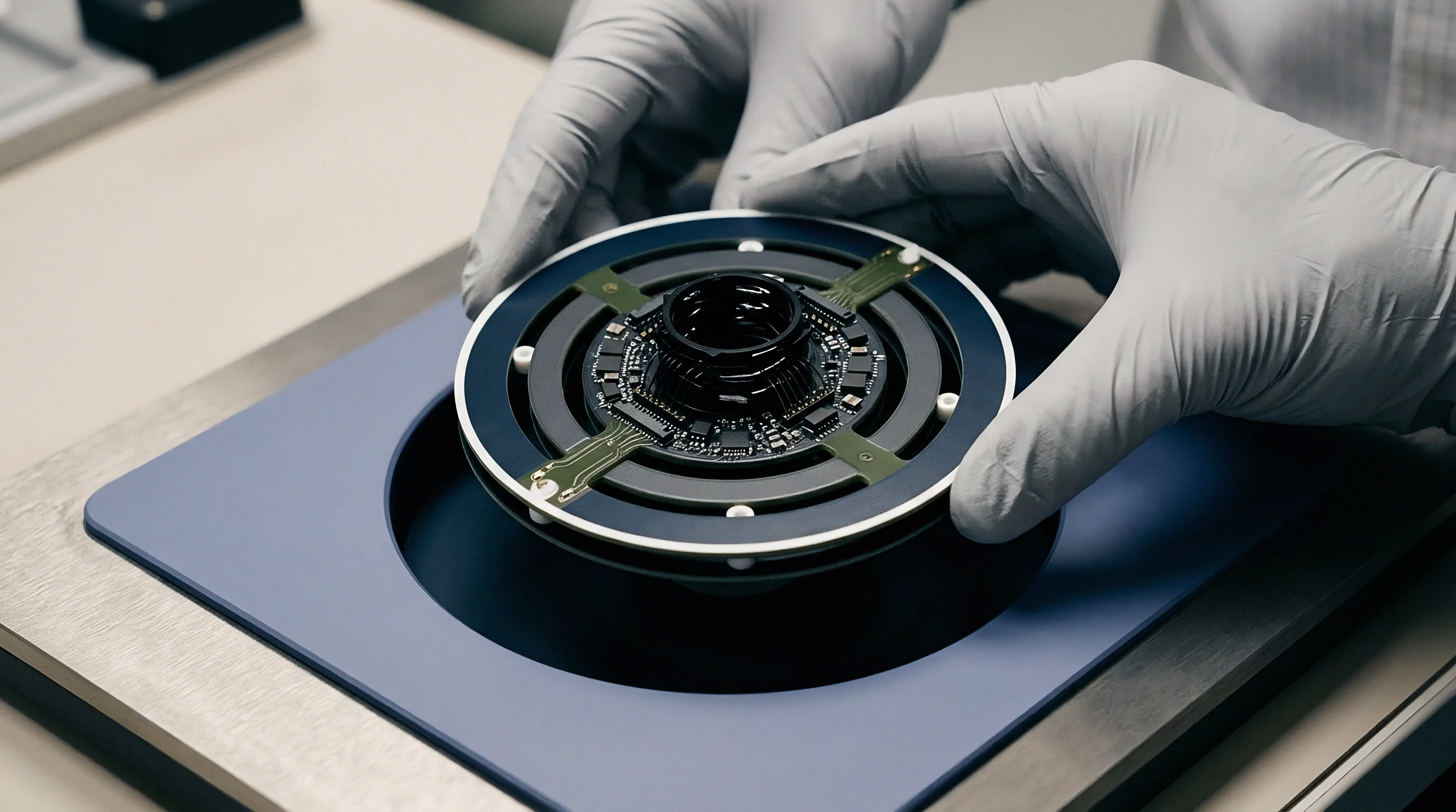

Margin
Manufacturing variations can quickly erode tight compliance margins. While prototype units built in development labs are hand-tuned, mass-production devices show component, board, and antenna variations across lots. Power amplifier tolerances alone can vary output power by up to 0.8 dB between batches.
In a system tuned close to SAR limits, that drift can push a production unit over legal exposure limits.
Antenna performance is sensitive to physical assembly variations. Small shifts in dielectric thickness, flex circuit placement, or glue volume change input reflection coefficients. These physical variances alter the near-field profile and shift peak exposure points, raising localized SAR even if conducted power remains unchanged.
Component manufacturing tolerances across high-volume power amplifier lots introduce up to 0.8 dB of conducted power spread, consuming the entire safety margin allocated in dynamic backoff lookup tables.
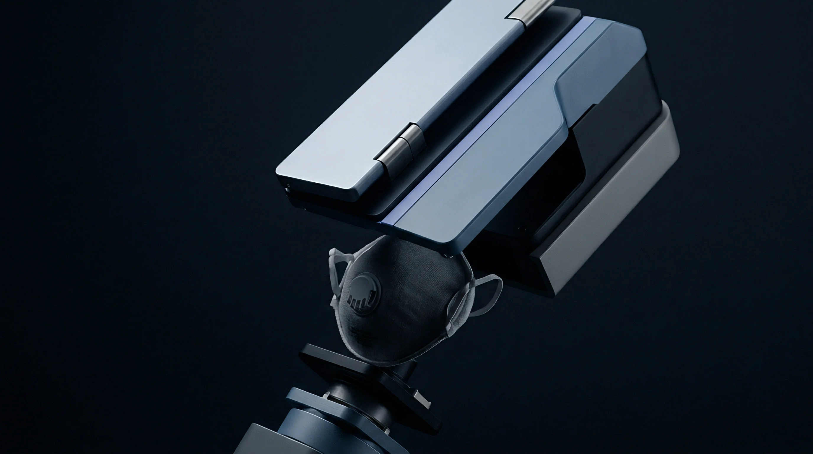
Production Variance and Antenna Coupling Drift
To protect against production spread, design teams build calibration guardbands into backoff state tables. If regulations mandate keeping spatial peak SAR under 1.6 W/kg over ten grams of tissue, factory calibration might target 1.3 W/kg instead. This 0.9 dB margin absorbs component variations, temperature drift, and housing tolerances without requiring field power cuts that degrade performance.
Improperly flashed test software yields invalid sliding window logs. Automated production stations program backoff offsets into non-volatile memory during final assembly. Calibration benches measure conducted output power at discrete trim points, writing gain compensation factors to each device before it leaves the factory.

Thermal Throttling and Operational Power Reserves
Thermal throttling operates alongside regulatory backoff algorithms. Under heavy processing loads, system thermal management throttles hardware power to protect silicon junctions from overheating. Because this thermal power reduction acts independently of regulatory backoff logic, it introduces secondary power changes.
If thermal throttling reduces transmit power below the level set by exposure backoff rules, the sliding window log records lower energy delivery. The algorithm can then use this exposure credit to permit higher power bursts once system temperatures cool, balancing thermal management against RF exposure limits.
Designers must coordinate thermal and exposure control loops to avoid power oscillation. Uncoordinated state machines can cause rapid power cycling that destabilizes RF links and drops throughput. Validating firmware control loops ensures smooth transitions across temperatures and battery voltages.
Establishing proper factory calibration guardbands allows design teams to absorb manufacturing drift while keeping link budgets high.