Quantifying Radiated Spurious Emission Measurement Uncertainty Expansion Factors in Millimeter Wave Test Chambers
Quantifying mmWave radiated spurious uncertainty expansion factors converts raw measurement deviations into defensible ninety-five percent compliance margins.

Budget
Standardized evaluation of high-frequency spurious emissions requires strict quantification of systematic errors across all physical hardware stages. At frequencies spanning 24 GHz to 110 GHz, free-space path loss and waveguide dispersion erode signal-to-noise ratios. A measurement receiver scanning for fifth-order harmonics of a 28 GHz carrier encounters baseline thermal noise floor limits and mixer conversion variations that distort radiated amplitude records.
Isolating the actual spurious level generated by a transceiver module demands a systematic accounting of every variance contributor between the radiator phase center and the spectrum analyzer detector.
Margins collapse above fifty gigahertz.
Measurement uncertainty in millimeter wave chambers compounds along the physical radio-frequency path. The combined standard uncertainty aggregates independent variance components through functional sensitivity models established under ISO/IEC Guide 98-3. Standard gain horn calibration tolerances, antenna cross-polarization misalignment, positioner sphere-of-error displacements, and harmonic mixer response variations each inject measurable dispersion into the observed signal power.
When a laboratory records a radiated peak at 56 GHz, that raw data point carries a confidence interval dictated by the algebraic expansion factor chosen for the test report.
ETSI TR 100 028 mandates deducting the test laboratory expanded uncertainty exceeding acceptable limits directly from the measured compliance margin.
Systematic versus Random Millimeter Wave Degradation
Path attenuation climbs past ninety decibels when test frequencies advance into E-band allocations. Systematic deviations originate from known physical mechanisms: cable insertion loss, calibrated horn gain curves, attenuator thermal drift, and downconverter non-linearities. Laboratories characterize these systematic elements through reference substitution measurements, storing correction vectors inside automated test software.
Random components stem from environmental fluctuations, turntable angular jitter, and local oscillator phase instability. Calculating the root sum of squares across these independent distributions establishes the baseline dispersion of the chamber setup.
Mixers produce spurious response artifacts.
Directivity drops off boresight.
| Error Source | Probability Distribution | Divisor | Standard Uncertainty (dB) | Sensitivity Coefficient |
|---|---|---|---|---|
| Antenna Gain Calibration | Normal (k=2) | 2.000 | 0.45 | 1.0 |
| Antenna Axis Alignment | Rectangular | 1.732 | 0.35 | 1.0 |
| Waveguide Mismatch Reflection | U-Shaped | 1.414 | 0.55 | 1.0 |
| Harmonic Mixer Conversion Drift | Rectangular | 1.732 | 0.80 | 1.0 |
| Cable Loss Flexure Variation | Rectangular | 1.732 | 0.60 | 1.0 |
| Turntable Radial Eccentricity | Rectangular | 1.732 | 0.25 | 1.0 |
| Chamber Quiet Zone Multipath | Rectangular | 1.732 | 1.10 | 1.0 |
| Receiver Amplitude Linearity | Rectangular | 1.732 | 0.40 | 1.0 |
Mathematical Aggregation via Welch Satterthwaite Formulations
Combining independent standard variances follows the root sum of squares method detailed in guide documents. Each component variance multiplies by the square of its partial derivative sensitivity coefficient. The combined standard uncertainty equals the positive square root of this sum.
When individual uncertainty terms possess differing degrees of freedom, calculating the effective degrees of freedom prevents underestimating the resulting confidence distribution. The Welch-Satterthwaite relation determines whether the expanded interval approximates a Gaussian curve or defaults to a wider Student t-distribution.
ETSI TR 100 028 Clause 4.2 dictates that test houses subtract measurement uncertainty figures that exceed documented limits from the measured margin before issuing a declaration of conformity.

Flange
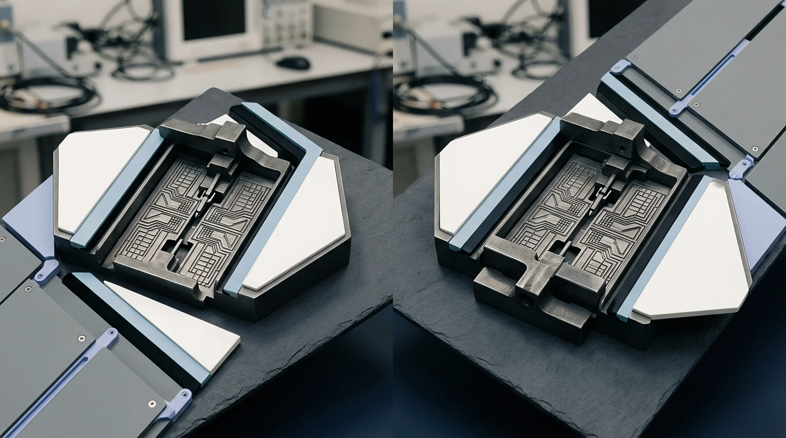
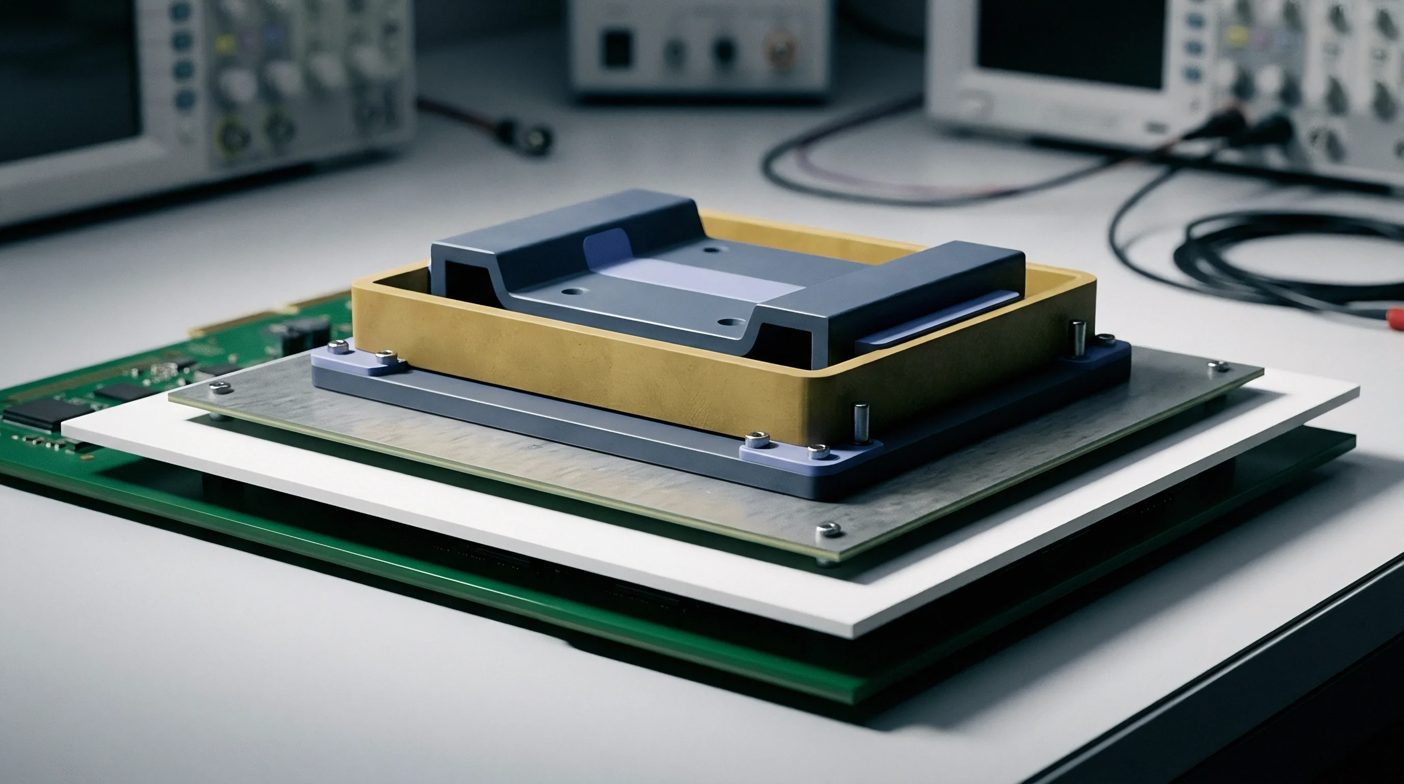
Mechanical waveguide interfaces operate as the primary transition point where millimeter wave power couples between antennas, mixers, and receivers. In WR-28, WR-15, and WR-10 bands, microscopic surface imperfections and misalignments generate substantial voltage standing wave ratios. An air gap of fifteen micrometers between mating waveguide sections creates reflections that manifest as frequency-dependent amplitude ripple across the receive chain.
Technicians tighten precision alignment pins to minimize transverse displacement during module substitutions.
Waveguide alignment degrades rapidly.
Alignment pins wear out quickly.
Where Do Harmonic Mixer Instabilities Corrupt Mmwave Spurious Scans?
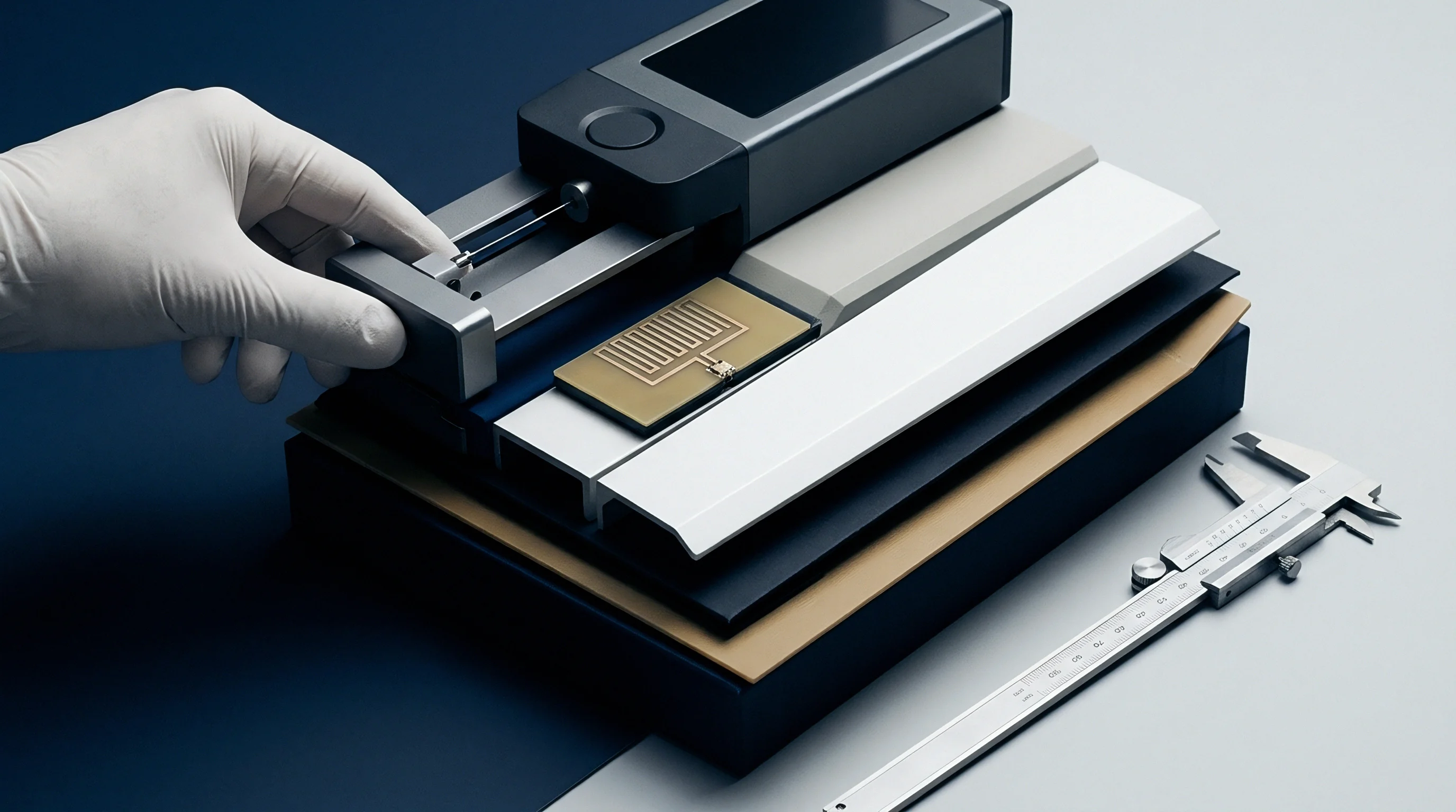
External downconversion modules introduce non-linearities and conversion losses that drift with local oscillator power variations. Harmonic mixers utilize the n-th harmonic of an internal reference source to downconvert signals in the 40 GHz to 110 GHz territory into the intermediate frequency range of the host spectrum analyzer. An unstable local oscillator drive drops mixer conversion efficiency unevenly across the frequency span.
The resulting conversion loss table, typically loaded as a static correction curve, diverges from physical realities when the laboratory ambient temperature shifts by five degrees Celsius.
Misaligned waveguide flanges convert transmission amplitude into phantom harmonic spurs long before cross-polarization isolation collapses.
Diode compression points inside harmonic mixers restrict dynamic range. Strong fundamental carrier signals leak past suppression filters into the mixer input port, creating intermodulation products that mimic device spurious emissions. Qualified operators introduce tunable waveguide band-reject filters or spatial notch cavities to suppress intentional transmit carriers before downconversion stages, preventing mixer overload artifacts from populating test data logs.
Cable Flexure and Rotary Joint Wear
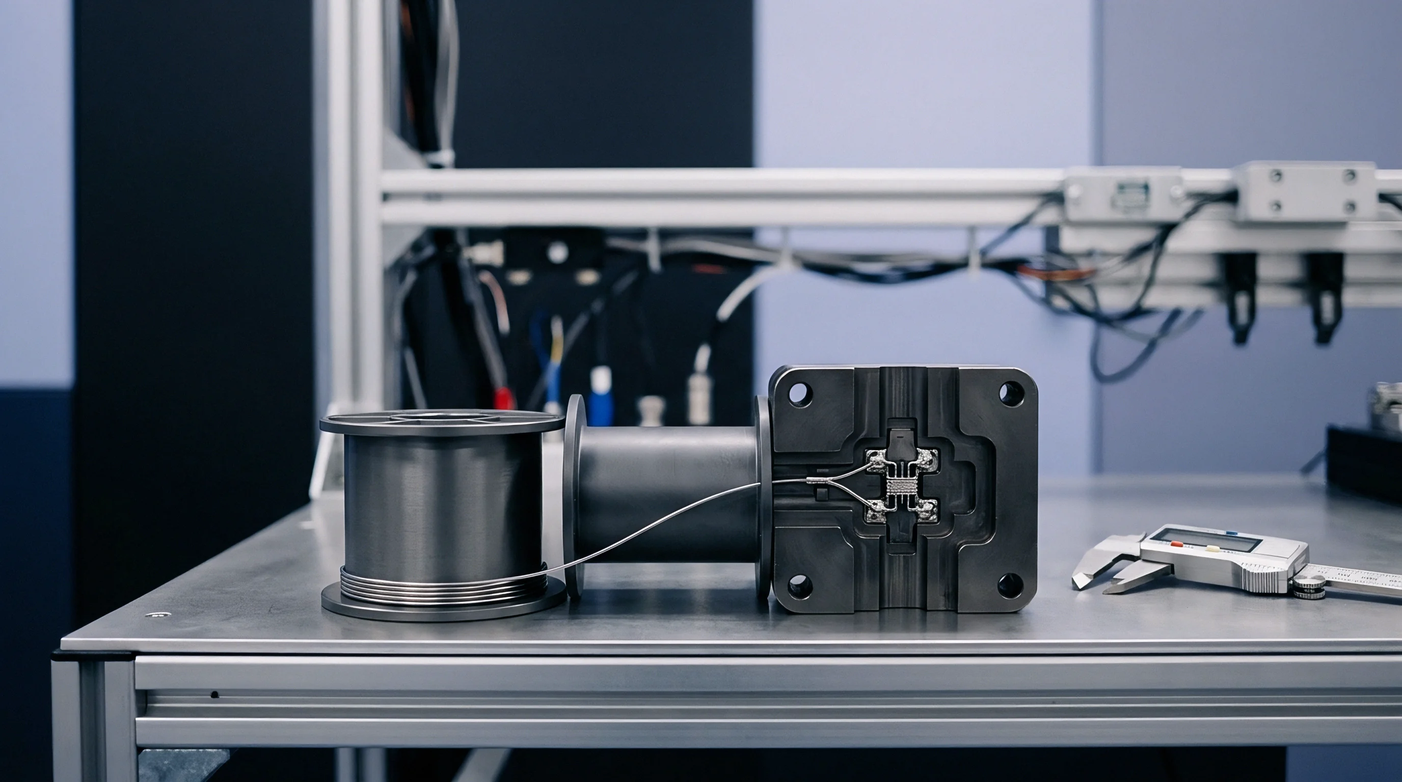
Coaxial transmission lines running to moving azimuth stages undergo continuous bending cycles during spherical spatial sweeps. Flexible 1.85 mm and 1.0 mm cable assemblies exhibit phase shifts and microphonic insertion loss deviations when twisted during continuous turntable rotation. High-frequency RF energy encounters dielectric compression inside flexed cables, yielding attenuation variations exceeding one decibel at 67 GHz.
Cable flex ruins measurement repeatability.
Physical deterioration mechanisms compromise high-frequency measurement setups across routine testing cycles:
- Waveguide Flange Cocking occurs when mounting screws apply asymmetric torque across precision contact planes, inducing reflection coefficients exceeding 0.15.
- Connector Pin Recession develops from over-torquing coaxial mating nuts beyond standard limits, displacing the center pin and causing intermittent impedance discontinuities above 40 GHz.
- Harmonic Mixer Diode Degeneration results from prolonged exposure to fundamental carrier leakage power, steadily eroding conversion linearity across high-order harmonic mixing products.
- Cable Armor Fatigue follows repeated continuous rotations of the turntable assembly, breaking interior shielding braids and inducing phase wobble across spatial scan sweeps.
The millimeter wave component vendor argued that factory calibration files held across three thermal cycles eliminate the need for daily receiver verification runs at the test bench.
Ripple
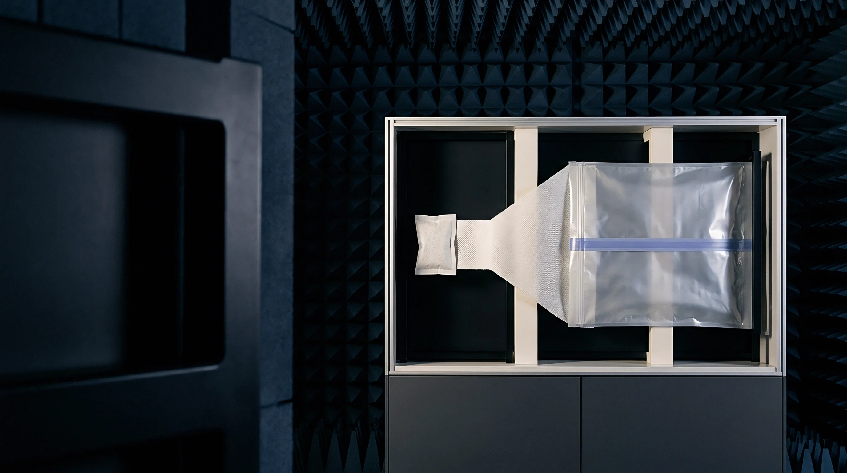
Chamber reflections superimpose stray wavefronts onto the direct line-of-sight propagation path. Inside anechoic and compact range enclosures, pyramidal carbon-loaded polyurethane foam absorbers attenuate incident millimeter wave radiation. At normal incidence, modern absorber cones achieve thirty-five to forty decibels of reflection loss at 28 GHz.
Oblique incidence angles common to side-wall and floor bounce paths reduce this attenuation to fifteen decibels, creating interference patterns within the designated quiet zone volume.
Phase ripple distorts peak amplitude readings.
Interference between direct and scattered wavefronts manifests as periodic amplitude ripple across the frequency sweep. When an automated test routine rotates the unit under test through 360 degrees of azimuth, spatial standing waves cause apparent power shifts unrelated to the actual emission pattern of the radio module. Bounding this uncertainty demands physical probing of the quiet zone across three orthogonal axes.
Mixer conversion loss variations above seventy-five gigahertz inflate combined standard uncertainty by 2.4 decibels when local oscillator drive power drops by a single decibel.
Quiet Zone Multipath and Absorber Degradation
Pyramidal carbon-loaded foam absorbers demonstrate rising specular reflection coefficients when incident wave angles depart from normal orientation. Absorber cone tips suffer physical bluntness and environmental humidity absorption over years of active chamber operation. At 90 GHz, a water film on deteriorated cone tips shifts the material dielectric constant, degrading return loss performance and transforming quiet zone reflections into significant systematic uncertainty contributors.
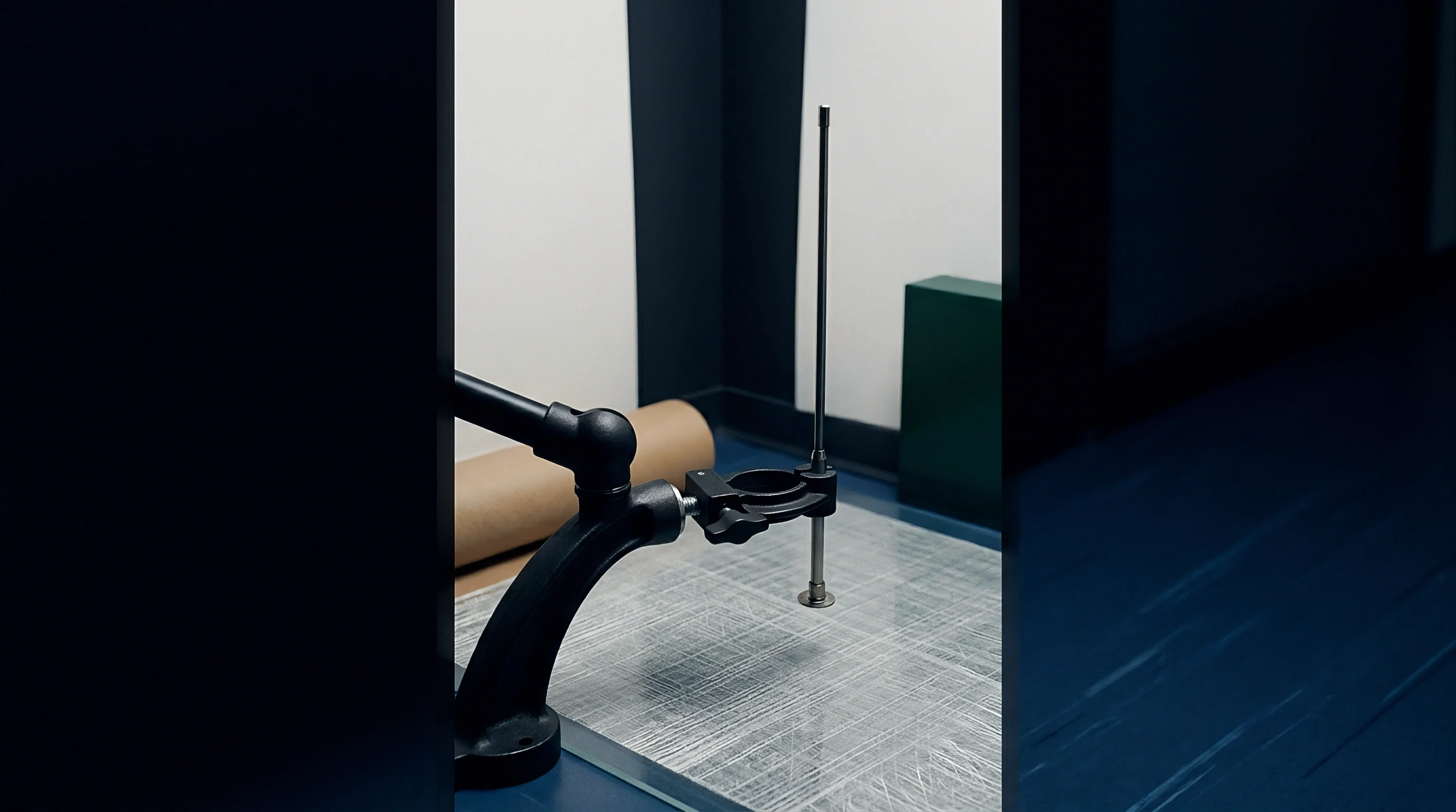
Chamber engineers run cylindrical and spherical field probing sequences to quantify quiet zone reflectivity envelopes across authorized bands. The field probe records spatial electric field variations across a volumetric cylinder encompassing the maximum dimensions of the equipment under test. Peak-to-peak ripple bounds within the quiet zone volume determine the rectangular uncertainty distribution assigned to spatial multipath.
Quiet Zone Spatial Validation Step Sequence
Field uniformity probing establishes the physical boundary where phase deviations stay within tolerable bounds.
- Position a standard gain horn antenna on the azimuth turntable at the center of the nominal quiet zone volume.
- Align the receive antenna bore-sight axis directly with the range feed horn using laser positioning targets.
- Sweep the local source generator across the operational frequency band while recording baseline transmission amplitude.
- Translate the probing antenna in fifty-millimeter increments along a linear transverse axis covering the quiet zone diameter.
- Record spatial amplitude and phase variations at each offset position across horizontal and vertical polarizations.
- Extract the maximum peak-to-peak amplitude deviation across the probe volume to derive the chamber quiet zone standard uncertainty component.
Whether future chamber qualifications can separate spatial multipath reflections from device internal antenna coupling at frequencies beyond one hundred gigahertz remains unresolved across standard bodies.

Spread
Translating combined standard deviations into expanded confidence intervals establishes the statistical boundary for compliance decisions. Under standard metrology rules, the combined standard uncertainty multiplies by a coverage factor, denoted as k, to yield the expanded uncertainty. A coverage factor of k=2 defines an expanded uncertainty interval corresponding to an approximate ninety-five percent level of confidence, assuming an underlying normal distribution with high degrees of freedom.
Narrow apertures require fine spatial steps.
When degrees of freedom fall due to sparse empirical calibration samples, the expansion factor scales outward according to the t-distribution. A test setup relying on three calibration runs cannot justify k=2 for ninety-five percent confidence; it requires k=2.48 to cover the equivalent statistical territory. Miscalculating this multiplier distorts the declared compliance margin, invalidating the test dossier during technical file reviews.
Why Does Far Field Distance Expand Path Loss Uncertainty?
Separation between the device under test and the measurement antenna directly sets the free space transmission attenuation. Millimeter wave modules utilize integrated antenna arrays exhibiting wide apertures. The Fraunhofer far-field boundary distance, calculated as two times the square of the antenna aperture diameter divided by the operating wavelength, pushes test distances beyond three meters for moderate array sizes at 60 GHz.
Path losses exceed ninety decibels.
Increasing test separation to satisfy far-field plane-wave criteria suppresses phase distortion across the receive aperture. The increased distance elevates path attenuation, driving low-level harmonic emissions below the receiver noise floor. Laboratories transition to Compact Antenna Test Ranges (CATR) using parabolic reflectors or near-field scanning techniques to compress physical separation while controlling phase taper errors.
| Frequency Band | Measurement Architecture | Combined Standard Uncertainty (dB) | Effective Degrees of Freedom | Coverage Factor (k) | Expanded Uncertainty (dB) |
|---|---|---|---|---|---|
| 24.25 GHz to 29.5 GHz | Direct Far-Field (1.5 m) | 1.85 | 48 | 2.00 | 3.70 |
| 24.25 GHz to 29.5 GHz | Compact Range (CATR) | 1.42 | 62 | 2.00 | 2.84 |
| 37.0 GHz to 43.5 GHz | Direct Far-Field (1.0 m) | 2.35 | 35 | 2.03 | 4.77 |
| 37.0 GHz to 43.5 GHz | Compact Range (CATR) | 1.75 | 54 | 2.00 | 3.50 |
| 57.0 GHz to 71.0 GHz | Direct Far-Field (0.5 m) | 3.10 | 22 | 2.07 | 6.42 |
| 57.0 GHz to 71.0 GHz | Compact Range (CATR) | 2.20 | 41 | 2.02 | 4.44 |
| 90.0 GHz to 110.0 GHz | Direct Far-Field (0.3 m) | 4.25 | 16 | 2.12 | 9.01 |
| Data represents empirical multi-lab validation averages compiled under 3GPP TR 38.810 methodology with isotropic radiators. | |||||
Coverage Factors and Fractional Degrees of Freedom
ISO Guide ninety-eight establishes multiplier values that convert combined standard uncertainty into expanded intervals corresponding to specific statistical coverage percentages. Test engineers calculate the variance of each input estimate alongside its assigned degrees of freedom. Components derived from physical calibration certificates carry known degrees of freedom, while engineering estimates based on rectangular bounds carry lower statistical reliability.
Accreditation audits penalize unverified assumptions.
Calculating the expansion factor demands rigorous verification of underlying input distributions:
- Calibration Certificate Entries supply baseline standard deviation figures with documented expansion factors, providing forty to one hundred degrees of freedom.
- Repeated Observation Series deliver empirical variances calculated from ten or more consecutive automated positioner sweeps, yielding direct degrees of freedom.
- Manufacturer Specification Tolerances define bounds without stated confidence intervals, requiring rectangular distributions divided by the square root of three.
- Mismatch Calculations employ transmission line reflection coefficients to generate U-shaped distributions divided by the square root of two.
Tighter quiet zones yield smaller expansion factors while wider measurement distances trade physical path loss against reduced phase distortion.
Friction
Test houses and equipment manufacturers face immediate commercial disputes when measured emission levels sit within the expanded uncertainty band of regulatory thresholds. Under FCC Part 30 rules, out-of-band emissions must remain below -13 dBm per megahertz. At 60 GHz, an expanded measurement uncertainty of 6.4 dB creates a substantial decision gray zone.
An observed emission peak of -15 dBm sits below the absolute regulatory ceiling, yet the expanded upper bound reaches -8.6 dBm, crossing directly into non-compliant space.
Re-spins destroy production margins.
Commercial contracts hinge on which party assumes the liability of measurement uncertainty. If the test plan enforces a shared-risk decision rule under ILAC-G8, an emission below the limit line constitutes a formal pass regardless of the uncertainty spread. If the filing targets regional markets requiring guard-banded compliance, the laboratory subtracts the entire expanded uncertainty from the regulatory limit, forcing the transceiver hardware to clear an effective barrier of -19.4 dBm.
A laboratory report showing compliance without expanded uncertainty calculations leaves the filing open to immediate rejection during regional audit reviews.
Shared Risk Rules and Guard Band Penalties
Accreditation guidelines define whether the laboratory or the applicant absorbs the risk of borderline out-of-band emissions. Shared risk conventions permit issuing a passing test report when the observed value sits below the legal limit, even if the ninety-five percent expanded confidence interval extends into non-compliant territory. This approach shifts consumer risk onto the regional spectrum management agency.
Positioners introduce mechanical wobble.
Guard-banded decision rules eliminate consumer risk by creating a conservative acceptance zone. The laboratory adds the expanded uncertainty figure to the emission reading. If the combined sum touches the limit line, the device receives a failing verdict.
A millimeter wave transceiver module designed with four decibels of engineering margin fails certification outright when tested inside a chamber carrying an expanded uncertainty of 5.5 dB.
Regulatory Market Filing Exposure
Regional certification authorities scrutinize out-of-band radiated performance reports to enforce compliance boundaries. Under European Radio Equipment Directive assessments, harmonized standards specify maximum permissible measurement uncertainty thresholds. When an accredited laboratory submits an RSE test report where the calculated expanded uncertainty exceeds the standard allowance, the notified body rejects the technical documentation file.
Test houses bill by shift.
Securing market grants across the United States, Europe, and Asia demands proactive test laboratory vetting. Sourcing teams verify chamber capabilities, receiver mixer ranges, and published uncertainty budgets before shipping pre-compliance production samples. A laboratory lacking WR-15 or WR-10 harmonic mixer calibration data inflates the expansion factor through conservative assumptions, turning a compliant hardware layout into an unmarketable inventory hold.
Failing to account for expanded measurement uncertainty during pre-compliance scans leads to rejected type examination certificates, repeated test campaigns, delayed market shipments, and commercial contract default penalties.