Statistical Process Control Requalification Protocols for Automated Assembly Lines
Line requalification demands baseline MSA verification below ten percent GRR followed by phase-gated subgroup testing before releasing automated lines.

Trigger
Automated SMT pick-and-place systems, robotic fastening cells, and high-speed fluid dispensing rigs operate within tight statistical limits. Once a disturbance breaks line continuity, historical control limits stop working. Plotting real-time process data against pre-disturbance baselines leads to false alarms or missed out-of-spec assemblies.
Requalification defines when historical baselines expire and when recalibration must take over.
Line disturbances fall into two main categories. Common cause variation is standard background noise ~ voltage micro-fluctuations, routine shop-floor temperature shifts, or component lot variances within vendor specs. Special cause events alter the physical geometry or kinematic transfers of the cell.
Tooling changes, nozzle swaps, optical sensor realignments, motor driver replacements, and major mechanical resets fundamentally shift the cell’s baseline variance. Requalification thresholds rely on physical disturbance boundaries rather than calendar intervals.
Background noise can mask progressive mechanical wear, rendering standard control limits useless. Requalification keeps those shifts from corrupting control charts.
Planned maintenance ~ like replacing a worn placement spindle on a multi-head gantry ~ shifts the mechanical center of mass and nozzle alignment vectors. Even with an identical OEM replacement part, micro-machining tolerances alter placement accuracy. Plotting post-maintenance offsets on a pre-maintenance Shewhart control chart violates a core SPC assumption: that the underlying process distribution stays stationary.
Stationarity requires the mean and standard deviation to remain stable until a documented change occurs.
Disturbance Classifications and Machine Boundary Shifts
Physical intervention on an automated line introduces mechanical changes that invalidate previous upper and lower control limits. Resetting a tool to nominal factory defaults does not restore the original distribution; every physical component carries distinct dimensional tolerances, friction traits, and dynamic responses under load. Replacing a lead screw on a positioning stage alters linear accuracy through minor lead variations along the thread.
Similarly, re-zeroing or retrofitting an optical encoder shifts the reference datum for all subsequent move commands.
| Disturbance Event | Physical Parameter Impact | SPC Invalidation Criteria | Requalification Mandate |
|---|---|---|---|
| Placement Head Nozzle Swap | Z-axis vacuum seat height and theta rotation concentricity offset | Subgroup mean shift exceeding 1.5 standard deviations from historic mean | Full 30-subgroup run-at-rate and short-term capability recalculation |
| Vision Camera Replacement | Field-of-view spatial scaling and pixel-to-millimeter conversion factor | Measurement variance shift yielding Gage R and R exceeding ten percent | Complete Measurement System Analysis and camera calibration protocol |
| Dispenser Solder Paste Lot Changeover | Rheological viscosity and volumetric flow rate under compression pressure | Three consecutive points beyond two standard deviations on range chart | Volumetric verification run with ten consecutive board test vehicles |
| Solder Reflow Heating Element Replacement | Thermal zone transfer coefficient and board soak temperature profile | Peak temperature shift greater than two degrees Celsius across zones | Nine-point thermocouple thermal profiling and conveyor speed lock |
| Robotic Arm Servo Drive Replacement | Encoder resolution, backlash compensation, and joint torque response | Cumulative theta axis drift exceeding 0.05 degrees over ten cycles | Kinematic trajectory recalibration and first-article dimensional check |
Unplanned line stoppages pose a less obvious threat to statistical process control. When a jam or emergency stop halts the line mid-shift, reflow oven thermal profiles drift and stencil printer solder paste thickens. Paste left exposed to ambient humidity for forty-five minutes during a mechanical fix loses solvent to evaporation.
This changes its shear behavior under the squeegee and skews print volume distribution. Restarting production without checking print volume capability almost guarantees downstream solder defects.
A process change that shifts the mean by more than one standard deviation destroys the statistical validity of pre-existing control limits.
Engineering Change Notifications that modify package geometry also invalidate active baselines. Dropping a passive component footprint from 0603 to 0402 alters thermal mass, feeder index increments, and optical centering algorithms. Automated inspection tools must update their measurement windows and defect thresholds accordingly.
Carrying historical control charts across a package geometry change masks machine calibration issues beneath component dimensional noise.
Miscategorizing disruptions leads to two main operational failures: operators either dismiss genuine process shifts as random noise, or they make unnecessary adjustments to a stable machine. Over-adjusting a stable system increases overall variance ~ classic machine tampering. Clear requalification protocols eliminate this guesswork by mapping specific statistical checks to each disturbance tier.
Operational Thresholds Mandating Line Stop and Re-Evaluation
Production halts become mandatory whenever process mean shifts cross defined standard deviation thresholds or critical mechanical assemblies are replaced. Line teams need clear quantitative triggers that stop production before non-conforming parts move downstream. These thresholds combine automated control chart rules with physical machine state monitoring.
- Statistical Out-of-Control Rules Standard Western Electric or Nelson rules ~ like a single point beyond three-sigma limits or nine consecutive points on one side of the center line ~ require immediate process isolation.
- Mechanical Component Substitution Replacing high-wear items such as placement nozzles, squeegee blades, dispense tips, or feeder modules demands a line halt and targeted verification.
- Software and Firmware Updates Changes to PLC code, motion trajectories, or vision inspection algorithms reset historical process baselines.
- Raw Material Specification Changeovers Switching raw material suppliers or running solder paste lots with viscosity deviations outside manufacturer specs requires re-establishing the process baseline.
Hitting any of these operational thresholds places the cell in quarantine. The line controller stops panel transport into the cell until a quality engineer completes requalification. Running boards through a quarantined line creates latent defects that pass visual inspection only to fail in functional testing or in the field.
Replacing components with original manufacturer parts during routine maintenance can still alter an optical head’s physical baseline, even when installed according to standard overnight procedures.


Gage
Uncorrected sensor drift corrupts statistical process control data. Automated lines rely on optical inspection, laser height sensors, and X-ray equipment to record real-time product dimensions. When the measurement tool carries excessive variance, the data reflects instrument noise rather than actual process variation.
Requalifying a line without first confirming measurement integrity guarantees flawed capability metrics.
Measurement System Analysis isolates the sources of variation inside an automated inspection cell. Total observed variance is the sum of part-to-part variation and measurement system variation. Measurement variation divides into equipment variation (repeatability under constant conditions) and appraiser or environmental variation (reproducibility across calibration cycles or shop-floor shifts).
Calibration drift skews mean values, and optics frequently degrade without obvious warning signs.
In high-speed environments, optical lenses accumulate flux residue, LED banks lose intensity, and camera mounts vibrate under rapid acceleration. These factors drive ongoing measurement drift. A vision system that measured solder ball diameters within five microns at commissioning can easily expand to a fifteen-micron spread after six months of multi-shift operation.
Requalifying the cell means separating instrument degradation from mechanical machine wear.
Vision System Calibration and Optical Alignment Controls
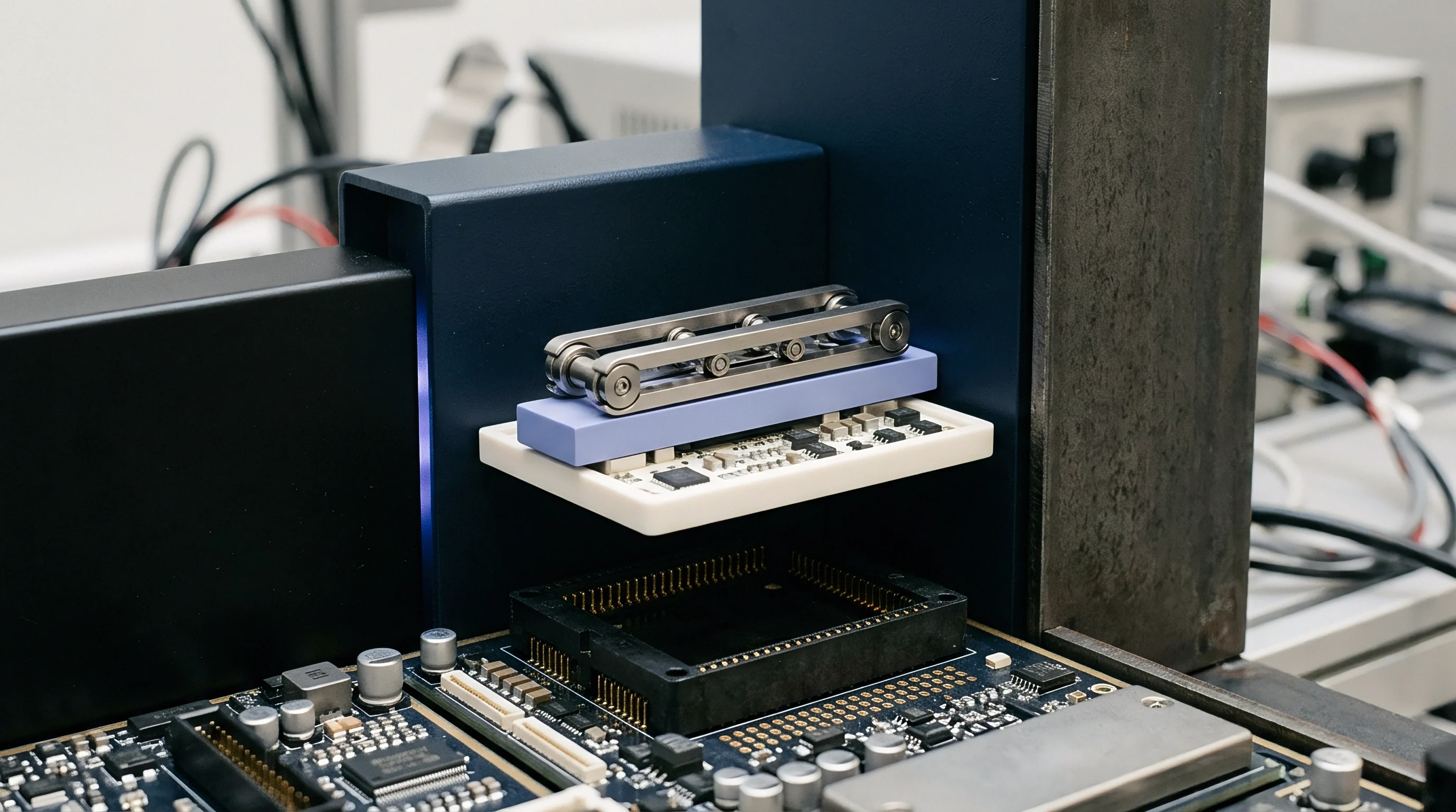
Automated optical inspection relies on stable lighting and precise focal distance to record accurate dimensions. Lens distortion ~ such as barrel or pincushion artifacts near image boundaries ~ skews spatial calculations. Without active software correction and physical calibration targets, features measured at the edge of the field of view will differ systematically from identical features measured at the center.
| MSA Metric | Acceptable Operating Zone | Marginal Operating Zone | Unacceptable Zone | Action Protocol |
|---|---|---|---|---|
| Percent Gage R and R (%GRR) | Below 10.0% | 10.0% to 30.0% | Greater than 30.0% | Halt line if %GRR exceeds 30%; recalibrate optics or sensors before proceeding |
| Number of Distinct Categories (ndc) | 14 or greater | 5 to 13 | Fewer than 5 | Low ndc indicates system cannot distinguish part variation; upgrade sensor resolution |
| Equipment Variation (%EV) | Below 8.0% | 8.0% to 20.0% | Greater than 20.0% | High EV reflects mechanical instability, sensor noise, or optical vibration |
| Appraiser Variation (%AV) | Below 5.0% | 5.0% to 15.0% | Greater than 15.0% | High AV indicates calibration discrepancies between operators or setup algorithms |
Evaluating an automated vision system requires a calibration target made of low-thermal-expansion quartz glass with chrome-deposited features of certified accuracy. The vision system scans the target across multiple grid coordinates, while software calculates pixel-to-millimeter factors and generates lookup tables to compensate for lens distortion. Measurement system acceptance limits are set at ten percent of total process variation.
High operational speeds shift baselines, sensor degradation hides real defects, and uncorrected measurement error quietly corrupts production runs.
Consider a practical evaluation on a surface mount line checking component alignment offsets. A quality engineer selects ten test coupons that span the full production tolerance range. The automated vision cell inspects each board ten times without operator intervention to isolate repeatability, then repeats the test across three separate shift changes and calibration cycles to assess reproducibility.
Gage Repeatability and Reproducibility must consume less than ten percent of the total process tolerance band to support valid statistical qualification.
If Percent Gage Repeatability and Reproducibility exceeds thirty percent, the measurement system cannot reliably separate good assemblies from bad ones. It will generate false alarms that halt healthy lines or allow out-of-spec joints to pass downstream. Requalification stops until technicians clean optical paths, replace aging LED elements, secure camera gantries, and re-verify calibration targets.

Can Automated Vision Systems Replace Manual Requalification Baselines?
High-speed cameras capture complex geometry far faster than tactile probes, but spatial distortion across wide fields of view introduces subtle measurement errors. Automated vision offers 100 percent screening, but the software relies on pixel thresholding logic. That thresholding depends on edge contrast, which shifts whenever PCB surface finishes change from Organic Solderability Preservatives to Electroless Nickel Immersion Gold.
Shifts in visual contrast alter the apparent edge of a solder pad or component lead without any actual change in physical dimensions. A system calibrated on matte solder masks will miscalculate pad edges on glossy masks due to specular glare. Relying entirely on vision inspection without periodic audits against a tactile coordinate measuring machine creates a false impression of stability.
Quality engineers use calibrated contact probes or laser profilometers to audit automated vision results during requalification. Cross-referencing optical data against absolute physical standards confirms that edge-detection algorithms stay accurate across material batches. Skipping these tactile checks lets software measurement artifacts corrupt historical process records.
Running an optical inspection system with an unverified Gage R and R leads straight to scrapped assemblies, unnecessary line halts, and contentious quality disputes between buyers and assembly vendors.
Sample
Statistical confidence during a restart depends on calculating subgroup sizes that detect small mean shifts quickly. Setting sample sizes arbitrarily creates severe statistical risk: too few samples allow major mean shifts to pass into full production, while oversized samples waste expensive materials and prolong downtime without yielding useful insight.
Initial sampling highlights hidden bias, subgroup selection governs fault detection, and any setup change resets historical baselines.
Requalification protocols separate short-term process capability (Cpk) from long-term process performance (Ppk). Capability measures what the line delivers over a narrow window where environment, material lots, and machine thermal states remain tightly controlled. Performance tracks overall output over days or weeks, incorporating ambient temperature swings, shift handoffs, and material batch transitions.
Subgroup Construction and Phase-Gated Restart Regimes
Phase-gated restarts divide initial production into discrete runs to track short-term variance before ramping back to full throughput. Rational subgroups form the foundation of this process. A rational subgroup consists of parts made under nearly identical conditions over a short interval, isolating inherent machine noise from between-subgroup variation driven by thermal drift or material changes.
Calculating the required subgroup size n requires defining alpha risk (false alarm probability), beta risk (probability of missing a shift), and the minimum physical shift delta the test must catch. Sample size calculation follows the non-central t-distribution formula:
Subgroup Size Calculation Equation: n = ( ( Z_alpha/2 + Z_beta ) / delta )^2
Where Z_alpha/2 is the standard normal statistic for two-tailed producer risk, Z_beta is the consumer risk threshold, and delta is the target shift size in standard deviation units. For a protocol designed to detect a 1.0 standard deviation shift in placement accuracy with five percent producer risk and ten percent consumer risk, the minimum subgroup size is eleven units across at least thirty consecutive subgroups.
Standard contract terms enforce a minimum short-term capability index threshold of 1.67 during initial line requalification runs.
A phase-gated release structures the transition from machine halt to full-rate production across defined verification gates, with each gate enforcing statistical criteria before advancing the cell.
- Stop the line and clear all partially processed assemblies from transport conveyors following any qualification-triggering disturbance event.
- Execute baseline mechanical zeroing, load verified master setup files, and run five blank test vehicles through the cell to confirm optical target acquisition.
- Process an initial pilot batch of thirty consecutive assemblies using certified reference components under steady-state operating parameters.
- Extract dimensional measurement data from automated inspection stations, calculate subgroup means and ranges, and verify process normality using the Anderson-Darling test.
- Compute the short-term capability index Cpk using within-subgroup standard deviation derived from the average moving range.
- Release the line to limited production status at fifty percent run-at-rate capacity if the calculated Cpk index exceeds 1.67.
- Collect five additional rational subgroups of ten units each during the limited production run and re-evaluate process performance index Ppk.
- Authorize full-rate production release when the calculated Ppk index maintains a value above 1.33 across three consecutive shifts.
Bypassing phase-gated verification invalidates capability calculations. Mixing assemblies produced during initial setup adjustments with those from steady-state operation inflates the standard deviation. That artificially inflated variance depresses Cpk values, causing capable machines to fail requalification audits.
Capability Index Verification across Short and Long Runs
Distinguishing short-term capability from long-term performance prevents releasing lines prematurely after maintenance. The capability index Cpk relies on within-subgroup standard deviation ~ calculated by dividing the average subgroup range R-bar by the unbiasing constant d2 or using pooled standard deviation across rational subgroups. This strips out between-subgroup drift to measure purely machine-level precision under steady conditions.
The process performance index Ppk uses overall sample standard deviation s, calculated across all individual measurements in the qualification run. This captures total process variance, including thermal drift, feeder vibration, component variations, and environmental shifts. A wide gap between Cpk and Ppk indicates that while the machinery itself is precise, the system suffers from environmental or material instability.
Consider an automated placement line undergoing requalification after an X-Y gantry linear motor driver replacement. Engineers collect thirty subgroups of five circuit assemblies each, measuring placement offset relative to pad centers. The upper specification limit is 50 microns, the lower specification limit is -50 microns, and the average subgroup mean is 2.1 microns.
The within-subgroup standard deviation calculated from R-bar/d2 yields 4.2 microns. Calculating short-term capability yields Cpk upper = (50 – 2.1) / (3 4.2) = 3.80, and Cpk lower = (2.1 – (-50)) / (3 4.2) = 4.13. The short-term Cpk value of 3.80 reflects exceptional mechanical precision over short runs.
However, overall sample standard deviation s across all 150 measurements yields 11.8 microns, driven by thermal expansion in the cold linear motor during restart. This gives a Ppk upper of (50 – 2.1) / (3 11.8) = 1.35 and Ppk lower of (2.1 – (-50)) / (3 11.8) = 1.47, resulting in a Ppk of 1.35.
The drop from 3.80 Cpk to 1.35 Ppk shows that thermal expansion in the motor positioning rail degrades placement accuracy as the gantry warms up. Qualifying the line solely on short-term Cpk would hide this drift, causing component misalignments after two hours of continuous operation. Requalification protocols must mandate a twenty-minute thermal warm-up before data collection begins.
IPC-9261 Section 4.2 requires demonstrating a short-term Cpk of at least 1.67 across thirty consecutive rational subgroups during requalification. Any modification to motion parameters resets historical capability databases completely.
Variance
Parallel heads on automated equipment introduce distinct statistical distributions that obscure overall line stability. Pick-and-place gantries, multi-spindle screw drivers, and multi-nozzle dispensers run multiple sub-tools simultaneously. Combining measurement data from six placement heads into a single control chart produces misleading averages: a failing head gets masked by five good ones, allowing defective assemblies to pass through unnoticed.
Multi-head equipment requires nested variance decomposition during requalification. Total variance splits into between-batch, between-head, and within-head components. When between-head variance dominates, the assembly station suffers from mechanical miscalibration between individual spindles or nozzles.
Adjusting the overall chassis will not fix localized head misalignments.

Hierarchical Subgrouping and Multi-Placement Head Deconstruction
Multi-spindle tools aggregate individual component placement errors into a combined output that conceals single-head calibration drift. Control charts for parallel processing stations must treat each placement head, spindle, or tip as an independent sub-process during requalification. Subgroups must isolate output by individual head before evaluating overall machine performance.
| Source of Variation | Sum of Squares (SS) | Degrees of Freedom (df) | Mean Square (MS) | F-Statistic | Variance Share % |
|---|---|---|---|---|---|
| Between Component Batches | 14.25 | 4 | 3.562 | 1.42 | 5.2% |
| Between Dispensing Heads | 185.60 | 3 | 61.867 | 24.65 | 68.4% |
| Within Head Repeatability | 80.32 | 32 | 2.510 | N/A | 26.4% |
| Total Variation | 280.17 | 39 | N/A | N/A | 100.0% |
A four-head automated fluid dispenser illustrates why nested variance decomposition is necessary. The system deposits conformal coating dots over IC pins, and quality engineers gather forty volume measurements across ten panels. A two-way ANOVA reveals that between-head variation accounts for 68.4 percent of total volume variance: Head 3 consistently deposits 18 percent more fluid than Heads 1, 2, and 4 due to wear in its valve seat.
Looking only at overall batch averages hides the wear on Head 3 because the four-head mean sits within global specification limits. Over time, that extra volume causes fluid bridging and electrical shorts in the field. Requalification protocols must evaluate individual head metrics before approving combined line control charts.
Mechanical wear introduces process skew, sudden shifts in variance require immediate line stops, and setup changes reset historical baselines.
Exponentially Weighted Moving Average (EWMA) control charts offer far higher sensitivity for detecting small, persistent mean shifts across parallel stations. Where standard Shewhart charts evaluate subgroup points independently, EWMA charts apply a weighted moving average that prioritizes the latest subgroup while retaining exponentially declining weights for older data. The EWMA statistic Z_t is defined by:
EWMA Statistic Equation: Z_t = lambda X_bar_t + ( 1 – lambda ) Z_t-1
Where lambda is the smoothing weight (typically 0.05 to 0.20), X_bar_t is the current subgroup mean, and Z_t-1 is the previous EWMA value. The tighter limits of EWMA charts catch micro-drift in individual placement heads long before traditional three-sigma Shewhart limits flag an out-of-control state.

Control Chart Limit Recalibration Mechanics
Recalibrating control limits after line maintenance requires separating steady-state baseline data from initial restart fluctuations. Engineers must recalculate center lines and upper/lower limits using fresh subgroup data gathered entirely under post-requalification steady-state conditions. Keeping historical control limits after major maintenance destroys SPC validity.
Control chart limits recalculate only after confirming process stability across thirty consecutive baseline subgroups.
Recalibrating control limits follows a step-by-step sequence to avoid contaminating the baseline.
- Data Screening Strip out initial setup pilot samples and warm-up assemblies from the recalculation dataset to ensure process stationarity.
- Normality Testing Run Shapiro-Wilk or Anderson-Darling tests to confirm post-intervention data fits a normal distribution.
- Subgroup Parameter Calculation Calculate subgroup means X-bar and ranges R or standard deviations s across new production samples.
- Center Line Assignment Set the grand mean X-double-bar as the new historical center line for process monitoring.
- Control Limit Derivation Calculate upper and lower control limits using statistical factors A2, D3, and D4 scaled strictly to post-maintenance variance.
New control limits must be locked inside the line execution system. Operators should never have software privileges to manually alter limits or suppress out-of-control alarms. Any undocumented manual change to control limits on an active line is a severe quality violation.
How far can parallel insertion heads drift out of alignment before localized variance invalidates global capability indices across multi-cavity tooling?

Scope
Contracts between module buyers and contract manufacturers often break down over who pays for unbudgeted line downtime. When an automated line stops for requalification after a tool failure or engineering change, costs accumulate fast ~ idle expenses run from three hundred to twelve hundred dollars per hour per assembly cell, before counting scrapped materials or late shipment penalties. Without clear scope boundaries in the manufacturing services agreement, recovery stalls while both sides argue over engineering fees and test vehicle scrap.
Turnkey assembly assigns primary manufacturing operations to the contract builder, but the buyer retains commercial ownership of product quality and design updates. A semi-custom model splits responsibilities: the buyer supplies firmware and schematics, while the factory handles process engineering and line balancing. In white-label sourcing, the factory owns the full process baseline and qualification routine.
Defining these operational boundaries upfront prevents commercial friction during unscheduled line stops.

Engineering Labor Allocation and Deliverable Boundaries
Technical statements of work must clarify whether the buyer or the contract manufacturer supplies statistical analysis personnel during restarts. When a major failure forces extensive requalification, friction quickly develops over engineering fees for statisticians, calibration specialists, and automation technicians. The statement of work should specify exact deliverable packages for each integration model.
A complete requalification transfer package requires five mandatory engineering deliverables prior to sign-off:
First Article Inspection Reports covering full physical dimensions across three consecutive production panels; raw MSA datasets with Gage R and R sheets and optical calibration files; process capability dossiers detailing Cpk and Ppk values with Anderson-Darling normality test p-values; baseline configuration files containing locked servo parameters, lighting levels, and feeder coordinates; and a formal sign-off sheet signed by the factory quality director and the buyer’s technical representative.
Downtime costs accumulate rapidly, but clear scope boundaries prevent commercial disputes whenever setup changes reset historical baselines.
Statements of work must divide requalification responsibilities clearly to prevent commercial impasses. When the contract manufacturer owns the turnkey scope, the factory absorbs routine requalification costs from component wear, equipment breakdown, or operator error. If the buyer issues an Engineering Change Notification that alters schematics or component selection mid-run, the buyer covers line downtime, consumed test vehicles, and engineering hours at agreed rates.

Commercial Mechanisms Governing Requalification Downtime Costs
Financial losses stack up quickly when automated lines sit idle awaiting statistical sign-off. Manufacturing contracts need clear commercial terms governing qualification delays and cost allocation. Ambiguous timelines lead to unbudgeted expense claims and damaged supplier relationships.
Contracts should specify maximum turnaround times for requalification after routine maintenance. If the contract manufacturer fails to complete phase-gated verification within eight hours of a planned tool change, downtime chargebacks apply to monthly invoices. Conversely, if the buyer delays dossier sign-off beyond four hours, the buyer compensates the factory for idle capacity at agreed standby rates.
Unambiguous statements of work bind line downtime financial remedies directly to statistical requalification sign-off milestones.
Tooling wear limits and component changeover thresholds belong in the purchase agreement. A solid contract defines labor rates, sample sizes, test vehicle limits, and statistical acceptance targets for each disruption tier. Establishing these expectations before line stops occur speeds up requalification, protects quality baselines, and keeps landed costs on budget.
A clear contract scope ties technical requalification steps directly to financial liabilities on the landed-cost sheet.