Calculating Multi-Camera Measurement Variance Breakdown in Automated Machine Vision Systems
Decompose multi-camera measurement variance into optical intrinsics, mechanical rig thermal drift, target artifacts, and Jacobian triangulation geometry.
Budget
Spatial measurement uncertainty in multi-camera vision platforms stems from distinct physical and mathematical factors. Optical distortion, pixel quantization, thermal drift along the baseline, triangulation geometry, and target localization errors combine into a total spatial variance tensor. In electronics manufacturing, battery pouch cell assembly, and powertrain dimensional gauging, precision inspection stations often fail site acceptance testing when integrators quote simple optical resolution as measurement uncertainty.
A five-megapixel sensor with a 0.01-millimeter ground sampling distance does not guarantee a 0.01-millimeter repeatability window across three dimensions.
Field-of-view geometry sets the physical lower bound for spatial measurement resolution. As convergence angles narrow, ray intersections degrade along the principal optical axes. The covariance matrix of a triangulated three-dimensional coordinate depends directly on camera focal lengths, principal point offsets, pixel pitch, and the relative spatial pose between optical heads.
When two cameras view an edge at an inclusion angle of 15 degrees, depth uncertainty along the epipolar baseline jumps by an order of magnitude compared to an orthogonal stereoscopic setup.
Baseline convergence angles under twenty degrees inflate depth coordinate variance by a factor of eight relative to planar pixel noise.
Measurement uncertainty modeling follows the ISO/IEC Guide 98-3 standard. Total measurement variance breaks down into Type A statistical repeatability terms and Type B systematic hardware bounds:
- Target Localization Noise arises from sub-pixel edge detection algorithms, illumination shifts, and sensor shot noise during feature extraction.
- Intrinsic Parameter Uncertainty covers residual radial distortion, tangential lens errors, and principal point shifts caused by lens barrel tolerance stack-ups.
- Extrinsic Mechanical Variance stems from vibration, thermal gradients across camera mounting bars, and bracket compliance under industrial acceleration loads.
- Refraction Index Fluctuations follow air density differentials created by nearby convection sources, process ovens, and automated climate control units.
Each source contributes variance terms that propagate through nonlinear triangulation equations. Integrators specifying turnkey vision cells need to establish variance budgets across all contributors before finalizing mechanical designs or sensor contracts.
Can Epipolar Geometry Absorb Thermal Expansion?
Linear thermal expansion in standard structural materials pulls camera sensors out of calibrated alignment over routine factory shifts. An extruded 6061-T6 aluminum mounting spar with a 600-millimeter baseline expands roughly 13.8 micrometers per degree Celsius. A temperature shift of five degrees moves stereo camera baselines by nearly 70 micrometers.
Left uncorrected, this physical displacement causes coordinate offsets that exceed process tolerances in semiconductor packaging and automotive battery module inspection.
Rigid-body stereo calibration algorithms cannot absorb structural baseline variations. Epipolar line constraints assume fixed spatial transforms between camera coordinate frames. When mounting spars expand, projection rays skew, producing artificial residual disparity that software pipelines misinterpret as workpiece warpage.
Inverting the stereo projection Jacobian shows that angular pitch shifts in a camera body cause measurement errors fifty times larger than pure translational baseline expansion. A three-arcsecond rotation of a single camera mount shifts planar feature coordinate calculations by tenths of a millimeter at a one-meter working distance.
Rig
Structural rigidity dictates baseline orientation integrity across multi-head optical cells. Welded steel pedestals offer damping properties and thermal expansion coefficients far better suited to stability than lightweight aluminum framing. Mounting vision cells directly on machine chassis subject to linear motor accelerations induces oscillations that can ruin spatial calibration within hours of starting production.
Cantilevered camera mounts only amplify high-frequency vibration coming from pneumatic actuators and conveyor belts.
Mechanical design reviews need to compare structural resonant frequencies against machine cycle speeds. Stiffening gussets, vibration isolation pads, and low-expansion materials like Invar or carbon-fiber composites preserve baseline geometry through changing operational cycles. Machined kinematic mounts allow technical staff to remove and reinstall camera heads without running full recalibration routines.
Flexing in mounting fixtures creates dynamic errors that standard single-image calibration procedures miss. Verifying dynamic measurement stability requires testing at simulated production speeds with accelerometers attached to each optical housing.
Rig stability requirements scale inversely with working distance. Long standoff distances magnify minute angular deflections at the sensor face into substantial spatial offsets at the object plane.
| Material Grade | Thermal Expansion Coefficient (ppm/K) | Elastic Modulus (GPa) | Density (g/cm³) | Relative Baseline Drift (μm/m·°C) |
|---|---|---|---|---|
| Structural Aluminum 6061-T6 | 23.1 | 68.9 | 2.70 | 23.1 |
| Structural Carbon Steel A36 | 12.0 | 200.0 | 7.85 | 12.0 |
| Cast Gray Iron Class 40 | 10.5 | 124.0 | 7.15 | 10.5 |
| Invar 36 Precision Alloy | 1.2 | 141.0 | 8.05 | 1.2 |
| Quasi-Isotropic CFRP Laminate | -0.5 to 1.5 | 95.0 | 1.55 | 1.0 |
Locking down mechanical structures prevents baseline calibration decay during production runs. Line managers often attribute drifting gauge measurements to image processing software when physical bracket deflection is the real issue.
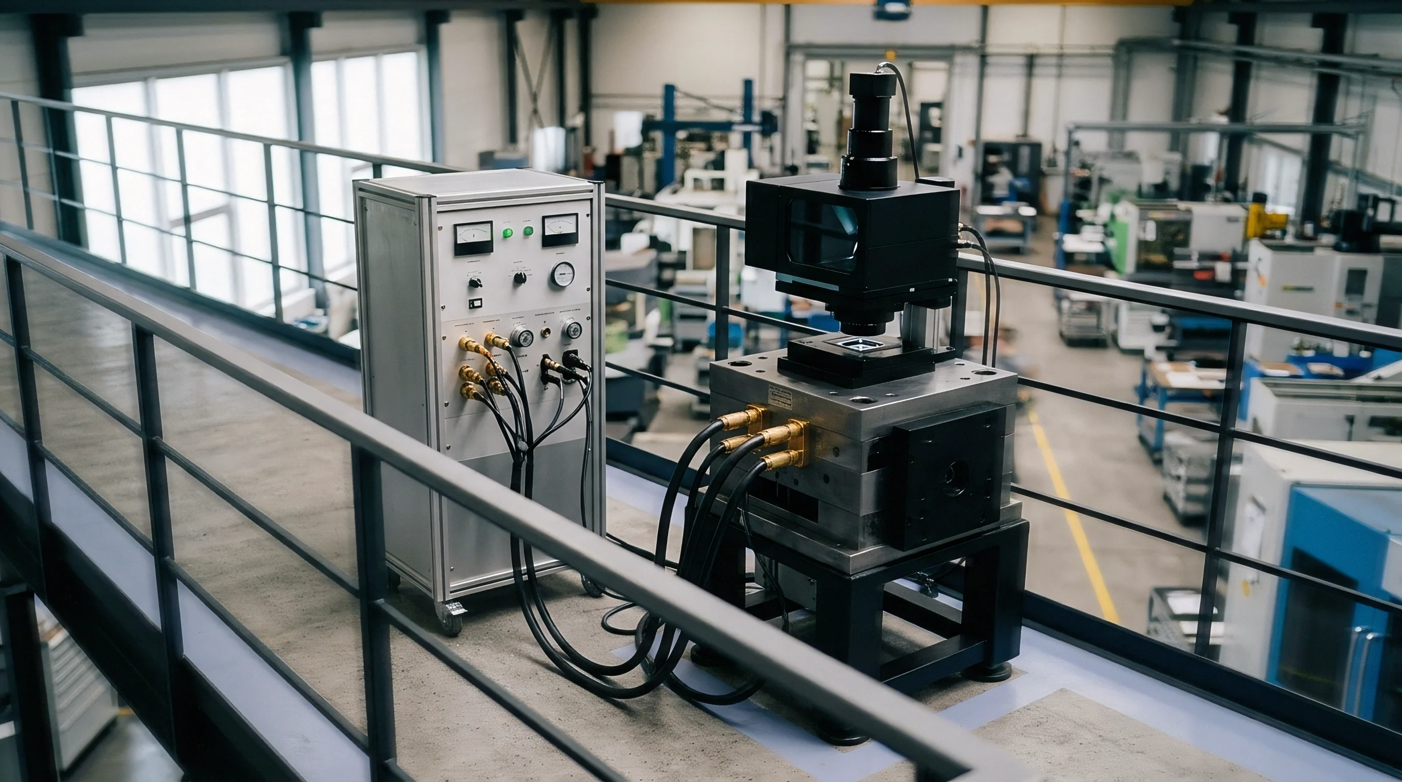
Stiffening the mounting assembly removes low-frequency resonance modes below 150 Hertz. Bolting cameras directly to granite risers or heavy box-section steel pillars minimizes cyclic deflections caused by nearby pick-and-place robots.
Propagation
Calculating overall spatial measurement variance requires propagating individual error distributions through the system of camera projection models. Forward projection maps world coordinates into camera sensor planes via extrinsic rotation and translation matrices followed by intrinsic transformations. Triangulation reconstructs three-dimensional points from intersecting light rays originating across multiple sensors.
The mathematical relationship between input feature point variance and output spatial variance relies on matrix differential calculus.
Let point vector X represent the true three-dimensional position of an observed target feature in global coordinates. Each camera c observes this point at sensor image coordinates u_c, subject to zero-mean Gaussian image noise with covariance matrix Sigma_u. The system forms an implicit observation equation f(X, u_1, u_2, u_n) = 0.
Applying the implicit function theorem yields the reconstructed spatial point covariance matrix Sigma_X through the system Jacobian matrices J_X and J_u:
Sigma_X = (J_X^T (J_u Sigma_u_total J_u^T)^(-1) J_X)^(-1)
Matrix J_X contains partial derivatives of the projection equations with respect to the three-dimensional world coordinates. Matrix J_u contains partial derivatives with respect to the observed image coordinates. Inverting this combined system propagates sub-pixel extraction uncertainty, lens distortion residuals, and camera pose uncertainties directly into three-dimensional coordinate confidence intervals.
A three-arcsecond rotation of an individual camera mount drives planar feature coordinate calculations off by tenths of a millimeter at a one-meter working distance.
Covariance propagation reveals clear directional anisotropy in multi-camera inspection envelopes. Planar variance parallel to sensor planes remains minimal, while variance along the primary depth axis expands dramatically. Adding three or four cameras at diverse viewpoints rounds out the error ellipsoid, replacing eccentric error distributions with spherical confidence regions.
| Camera Setup | Convergence Angle | Image Noise (Pixels) | Planar Variance (X/Y, μm) | Depth Variance (Z, μm) |
|---|---|---|---|---|
| Dual-Camera Stereoscopic Narrow | 15° | 0.05 | 4.2 | 32.8 |
| Dual-Camera Stereoscopic Wide | 45° | 0.05 | 3.8 | 10.1 |
| Dual-Camera Orthogonal Setup | 90° | 0.05 | 3.1 | 3.2 |
| Tri-Camera Symmetrical Cluster | 60° | 0.05 | 2.4 | 4.1 |
| Quad-Camera Tetrahedral Array | 70° | 0.05 | 1.8 | 2.3 |
Multi-camera setups reduce total spatial variance by adding redundant geometric constraints. Moving from two to four cameras cuts spatial variance by more than fifty percent while eliminating single-camera line-of-sight occlusions on complex workpieces.
Covariance cross-coupling terms indicate high sensitivity to extrinsic calibration accuracy. A minute misalignment between optical centers introduces correlated measurement bias across entire production batches.
Calculating the full covariance matrix lets system designers establish reliable statistical process control limits without relying on guesswork or optimistic calculations. Process engineers use these figures to verify whether an optical layout meets target capability metrics like Cp and Cpk.
Artifact
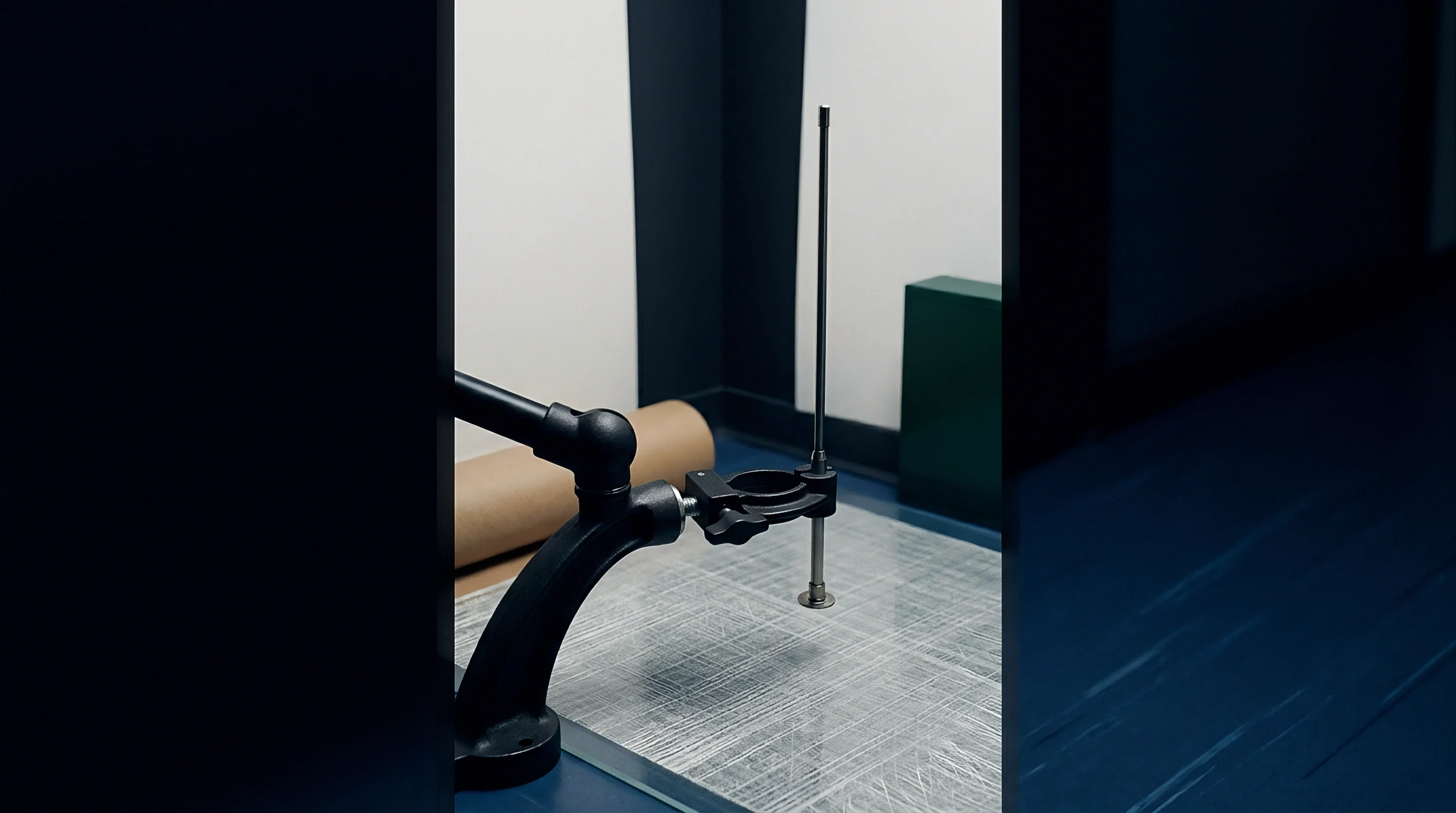
Traceable spatial calibration depends entirely on the physical precision of the calibration artifact. Integrators often buy commercial printed glass or ceramic checkerboards that lack certificates from a national metrology institute. A plate with nominal 10-millimeter grid spacing and uncertified thermal expansion rates introduces systematic scaling bias across the multi-camera field of view.
Calculating variance breakdowns requires isolating artifact manufacturing tolerances from vision sensor noise.
Precision targets use low-expansion ceramic, quartz, or soda-lime glass substrates etched with chrome photolithography patterns. Dot arrays, AprilTags, and ChArUco patterns offer different levels of extraction accuracy and resistance to partial occlusions during in-situ calibration routines. Certified feature pitch tolerances on high-grade optical targets typically hold within 0.5 micrometers across a 300-millimeter plate.
Optical targets lacking calibration certificates from accredited metrology bodies forfeit ISO 17025 compliance across automated inspection lines.
Whose Calibration Target Dictates the Traceability Chain?
Disputes frequently arise during factory acceptance testing when a buyer inspects parts with a coordinate measuring machine while the integrator calibrates using an uncertified dot grid. The resulting dimensional discrepancy usually stems from target pitch errors rather than optical triangulation faults. Traceability standards require every calibration plate to carry a certificate linking its feature positions to national length standards through an unbroken chain of measurements.
System integrators follow a structured sequence when qualifying calibration artifacts for high-tolerance automated inspection cells:
- Substrate Material Selection matches thermal expansion properties to ambient factory floor conditions, using quartz or low-expansion glass in temperature-variable test cells.
- Pattern Geometry Certification documents exact feature coordinates using contact coordinate measuring machines accredited under ISO 10360-2 metrology standards.
- Feature Extraction Validation tests sub-pixel circle-center and saddle-point edge detection algorithms against simulated non-uniform lighting fields to quantify thresholding bias.
- Recalibration Scheduling Intervals establish mandatory third-party optical recalibration dates to monitor surface wear, scratch accumulation, and substrate warping over operational lifetimes.
Neglecting target recalibration cycles compromises measurement integrity. Scratched chrome patterns shift detected feature centroids by tenths of a pixel, corrupting intrinsic lens distortion models during routine daily recalibrations.
Precision artifacts must sit in protective temperature-controlled storage when not deployed inside machine envelopes. Dust, oil mists, and solvent residues degrade edge contrast and distort sub-pixel feature detection.
Scope
Commercial agreements for automated machine vision systems must define the statistical boundaries of measurement variance breakdowns. Turnkey procurement specifications that demand dimensional inspection accuracy without defining confidence intervals, part surface conditions, temperature swings, and cycle times invite contractual disputes. Suppliers quote high capability metrics assuming pristine, flat, static parts at exactly 20 degrees Celsius, but production lines handle stamped, reflective, oily parts vibrating down index conveyors.
A thorough statement of work establishes distinct engineering line items for optical simulation, ray-tracing covariance analysis, dynamic vibration testing, and traceable calibration artifact delivery. Buyers who bundle these tasks into generic integration fees lose sight of the root causes of dimensional measurement failures during final runoff. Defining acceptance thresholds through gauge repeatability and reproducibility ratios establishes clear boundaries between mechanical variance and optical subsystem uncertainty.
The contract framework assigns financial responsibility for recalibration fixtures, reference standards, and software maintenance. System pricing shifts substantially depending on whether the integrator delivers documented open-source calibration pipelines or proprietary compiled binaries that lock the end user into exclusive service contracts.
Industrial vision procurement terms reflect explicit division of labor across mechanical structures, optical hardware selection, software algorithms, and ongoing metrological traceability through production runs.