W-Band Free Space Permittivity Extraction Fundamentals for Polymers
W-band free-space quasi-optical permittivity extraction requires sub-micron alignment and time-domain gating to ensure polymer radomes meet global type approvals.

Optics
Calculating complex permittivity between 75 GHz and 110 GHz requires strict control over how millimeter-wave signals propagate. Free-space quasi-optical setups avoid the mechanical stress and air-gap errors of rectangular waveguide clamps, but wave divergence presents its own challenges. Across the W-band, wavelengths range from 4.0 mm down to 2.7 mm.
At this scale, standard far-field horn approximations fall apart unless focused optics shape the beam across the polymer sample plane.
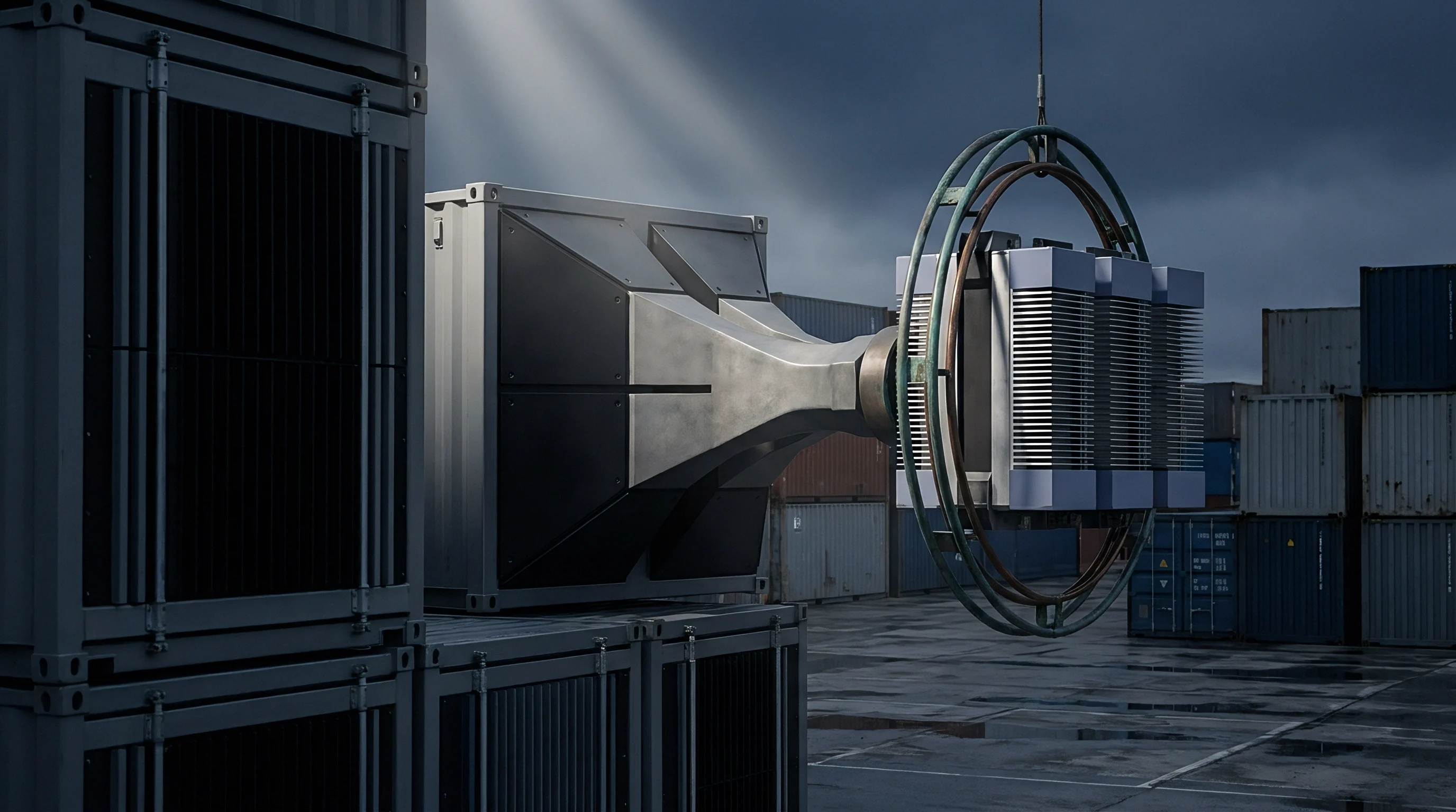
A quasi-optical bench converts the spherical wavefront leaving a scalar horn antenna into a localized Gaussian beam. Two refractive lenses ~ usually machined from high-density polyethylene or polytetrafluoroethylene ~ focus the energy to a waist at the sample position. This waist radius marks where the phase front stays flat.
If the phase front curves across the sample plane, it adds parasitic phase delays to the measured transmission coefficient and corrupts the real permittivity calculation. Matching the focal plane to the center of the polymer slab keeps this phase distortion low.
The physical size of the polymer specimen is mostly set by diffraction requirements. Any energy leaking past the edges creates multipath interference at the receiver lens. Keeping edge diffraction below negative forty decibels requires a sample width at least three times the three-decibel beam spot diameter.
At 77 GHz, a bench using fifty-millimeter aperture lenses with a one hundred millimeter focal length gives a waist diameter around twelve millimeters. Polymer specimens therefore need a clear aperture of at least thirty-six millimeters in diameter or side length.
Misaligned bench optics show up as an artificially elevated loss tangent.
Extraction equations assume a plane wave at strict normal incidence. Mechanical tilt creates an oblique path through the material, shifting phase accumulation away from the calibrated free-space baseline. Verification relies on an optical mirror placed in the sample holder.
A red laser aligned down the center axis of both horn antennas checks perpendicularity. Angular deviation has to stay under one-tenth of a degree to avoid polarization mixing and cross-polarization leakage across the W-band aperture.
Raw measurement validity depends heavily on phase stability in the Vector Network Analyzer extension modules. Frequency extension heads multiply the analyzer’s base frequency up to the 75-110 GHz range. Thermal drift inside these active heads shifts their internal phase response during a run.
Stabilizing the setup requires at least ninety minutes of electronic warm-up, along with temperature-stabilized module housings, before taking baseline calibration scans.

Gaussian Beam Waist Optimization across W-Band
Beam contours shift across the 35 GHz span of the W-band. At 75 GHz, the longer wavelength spreads the beam waist out, demanding larger sample apertures to avoid edge spillover. At 110 GHz, the beam tightens, concentrating energy on a smaller area.
Bench design has to account for the lowest frequency in the band so diffracted energy stays suppressed throughout the entire sweep.
The maximum practical polymer thickness depends on the Rayleigh range, which is the axial distance over which the beam’s cross-sectional area doubles from its waist. For a six-millimeter waist radius at 94 GHz, the Rayleigh range is about thirty-seven millimeters. Samples thinner than one-tenth of that distance sit in a virtually flat phase front, satisfying the boundary equations used for single-reflection and single-transmission calculations.

Refractive Lens Selection and Focal Geometry
Lens geometry dictates both spot size and focal depth. Plano-convex profiles introduce less internal spherical aberration than symmetric bi-convex lenses when focusing output from scalar feed horns. High-density polyethylene works well here as a low-loss dielectric with a stable refractive index near 1.53 across the W-band.
Machining tolerances on the lens curvature radius must be held tighter than twenty micrometers to keep the phase profile symmetric at the waist.
Mounting fixtures for polymer samples need non-reflecting frames. Aluminum plates coated with millimeter-wave absorber foam stop ambient scattering into the receiver. The positioning stage sits on a precision linear rail with sub-micron optical encoders.
This level of position control allows precise phase baseline zeroing during open-path calibration.
Focusing precision sets how reliably measurements repeat. When setting up a quasi-optical rail for W-band material testing, mechanical alignment must be set before running calibration scans. If the rails flex under the weight of the receiver module, calibration validity drops immediately.

Gating
Raw frequency-domain S-parameter traces in the W-band bundle together the target polymer response, internal module reflections, horn mismatch ripple, and room scattering. Separating the specimen’s actual response takes vector calibration combined with time-domain signal processing. Without filtering, transmission measurement ripple can hit half a decibel, introducing clear errors into extracted real permittivity values.
Free-space Thru-Reflect-Line calibration establishes the primary error coefficients for the system. The Thru standard aligns the two lens horns directly with no sample in place. The Reflect standard uses a flat metal plate at the focal plane as a phase reference.
The Line standard shifts one horn assembly along the optical axis by one-quarter wavelength at the band midpoint ~ at 92.5 GHz, that displacement is roughly 0.811 mm. How accurately the positioner sets this Line standard dictates baseline phase uncertainty across the sweep.
Time-Domain Gating applies mathematical filtering to separate the sample’s impulse response from stray environmental reflections. Vector network analyzers convert frequency-domain broadband data into the time domain using an Inverse Fast Fourier Transform. The resulting impulse response shows clear peaks for reflections from the front lens face, the front and rear surfaces of the sample, and downstream receiver optics.
Choice of window function governs gate resolution and side-lobe truncation. A Minimum Kaiser-Bessel window gives a reasonable balance between main-lobe width and side-lobe attenuation. If the gate is too narrow, it clips the extended impulse tail of low-loss, high-permittivity polymers, distorting the transformed spectrum.
If it is too wide, secondary reflections from horn feed transitions leak back in, adding periodic ripple to the frequency data.
Operators sometimes argue that un-gated free-space measurements are fine as long as absorber foam surrounds the fixture path. That assumption overlooks multiple internal reflections between the horn and lens, which travel directly along the optical axis regardless of surrounding foam.
Time-Domain Signal Processing Sequences
- Run a full two-port, two-receiver vector calibration over 75 GHz to 110 GHz, averaging 64 sweeps per standard.
- Place the polished metal calibration plate at the focal plane and record the baseline reflection impulse in the time domain.
- Measure the width of the main reflection peak to set the minimum passband duration for the gate envelope.
- Replace the metal plate with the polymer specimen, keeping it flush against the reference mounting pins.
- Transform S11 and S21 data to the time domain, centering the bandpass gate on the polymer impulse response.
- Apply the Kaiser-Bessel gate function, cutting off temporal data lower than negative thirty-five decibels relative to the main peak.
- Transform the gated time-domain response back into the frequency domain to produce clean magnitude and phase curves.
Residual Flutter and Boundary Noise Truncation
Truncation errors show up as artificial oscillations in calculated loss tangents. When a gate cuts off internal Fabry-Perot reverberations inside low-loss polymers, the frequency-domain transmission curve loses phase balance. A properly sized gate covers at least three full round-trip delays inside the slab.
In a two-millimeter thick polymer with a real permittivity of 2.56, a double-pass transit takes about 21.3 picoseconds. The gate width must therefore span at least eighty picoseconds to capture four full passes.
Filtering algorithms must keep phase linear during conversion. Any non-linear phase distortion from poor windowing shifts the slope of the transmission phase curve. Because that slope maps directly to real permittivity, linear-phase digital filters are essential for millimeter-wave extraction.
Air currents in the lab can shift optical path lengths during long test runs. Room temperature shifts change the refractive index of ambient air, altering the path length by several micrometers over an hour. Enclosing the quasi-optical bench in an acrylic housing stabilizes air density and preserves calibration integrity across multi-sample runs.


Slab
Physical sample quality sets the ultimate accuracy limit for W-band permittivity extraction. Extraction models assume homogeneous, isotropic, flat, parallel-faced dielectric slabs. Imperfections in the specimen translate directly into permittivity errors, which can mask subtle material losses or generate fake dispersion profiles.
Thickness variation across the illuminated area dominates the uncertainty budget. At 100 GHz, a quarter-wavelength inside a polymer with a dielectric constant of 2.25 is about 0.50 mm. A thickness change of just ten micrometers across the beam spot introduces over two degrees of phase variation in transmission.
Precision grinding or diamond turning can produce slabs with parallelism held within five micrometers over a fifty-millimeter face.
| Polymer Family | Nominal Thickness (mm) | Thickness Variance (µm) | Measured Real Permittivity | Loss Tangent (10^-4) |
|---|---|---|---|---|
| Polytetrafluoroethylene (PTFE) | 3.175 | ±3.2 | 2.06 | 4.2 |
| Liquid Crystal Polymer (LCP) | 1.500 | ±2.1 | 3.14 | 21.5 |
| Polyether Ether Ketone (PEEK) | 2.000 | ±4.5 | 3.08 | 34.0 |
| Cyclic Olefin Copolymer (COC) | 2.500 | ±1.8 | 2.35 | 6.8 |
| Polycarbonate (PC) | 1.500 | ±5.0 | 2.82 | 85.0 |
Surface roughness causes parasitic phase delays and local scattering loss. When high-frequency waves pass through a micro-rough surface, any root-mean-square roughness exceeding one-twentieth of the wavelength in the material causes backscattering that drops transmission magnitude. For W-band work, surfaces should be polished better than 0.8 micrometers RMS.
Polymers absorb ambient moisture, which alters their dielectric properties. Water has a very high real permittivity and loss factor at 77-110 GHz because of dipolar relaxation tails. Even 0.1 percent absorbed water by weight noticeably raises the loss tangent of low-loss polymers like PTFE or COC.
Standard preparation involves vacuum baking specimens at sixty degrees Celsius for twelve hours and storing them in a desiccator until mounting.
A sample thickness deviation of 15 micrometers at 77 GHz creates an uncalibrated phase error over 12 degrees.
Substrate anisotropy adds another variable. Extruded polymer sheets often align molecular chains along the machine direction differently than the transverse direction, producing uniaxial or biaxial dielectric behavior. Free-space setups with linearly polarized scalar horns only measure the permittivity component aligned with the incident electric field vector.
Rotating the sample ninety degrees in its mount reveals transverse variations, which matter when designing radome walls.
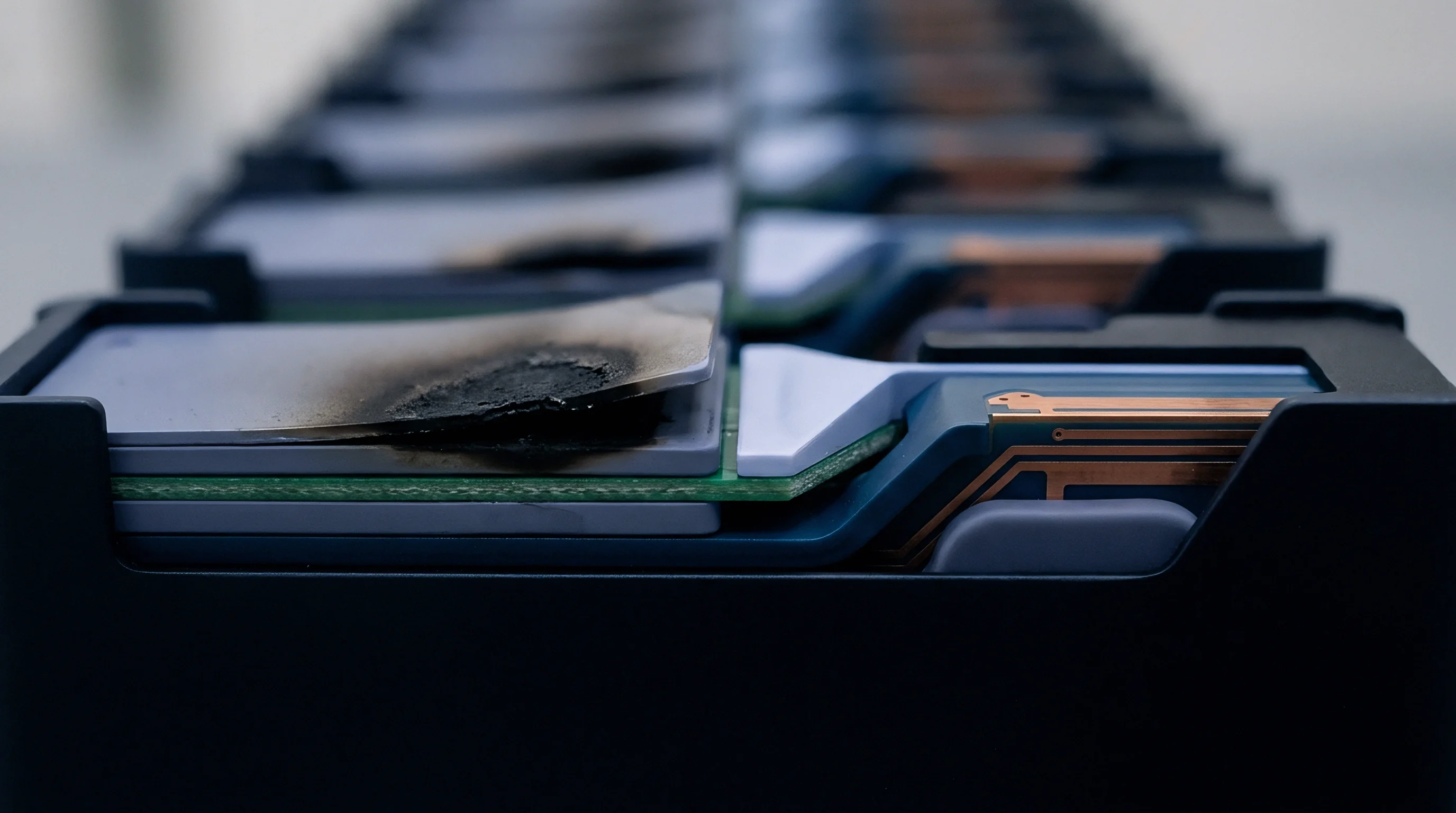
Polymer Selection and Physical Machining Constraints
- Polytetrafluoroethylene Formulations offer very low dielectric loss across W-band, but tend to creep or cold-flow when clamped mechanically.
- Liquid Crystal Polymers show strong dimensional stability and low moisture absorption, though they exhibit significant dielectric anisotropy between in-plane and out-of-plane directions.
- Cyclic Olefin Copolymers combine optical clarity with ultra-low loss tangents, making them good reference materials for quasi-optical validation scans.
- Polyether Ether Ketone Grades provide high mechanical rigidity and thermal resistance, but their higher dissipation factors require careful gate positioning in the time domain.
Clamping pressure needs careful control during mounting. Overtightening screws deforms soft polymer edges and introduces internal stresses that shift local density. Variable density alters the local refractive index across the illuminated area, hurting repeatability when samples are reloaded.
Ignoring surface non-parallelism leads to nonsensical extraction outputs, including negative loss tangents or artificial dispersion curves across the band.
Solvers
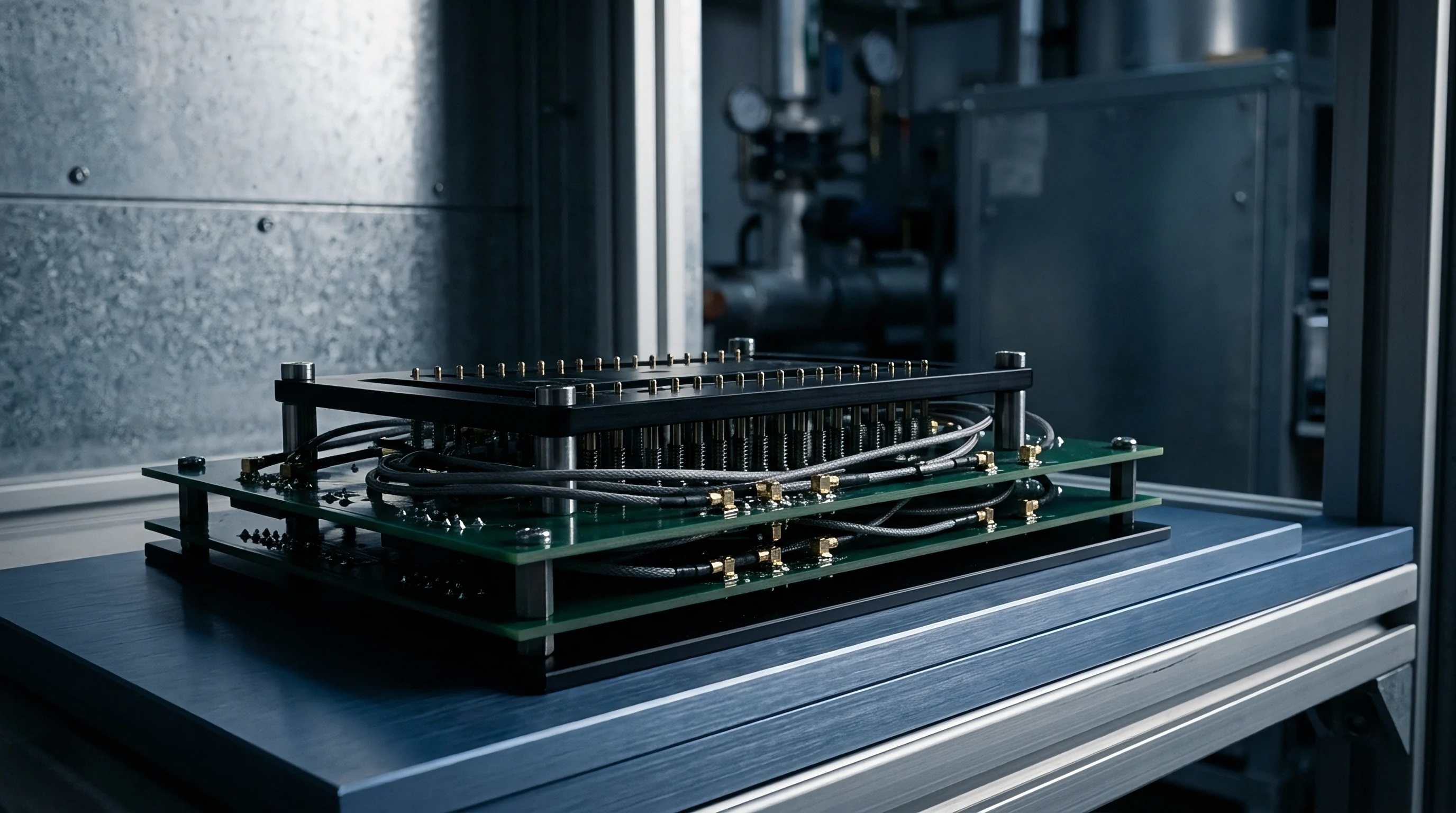
Converting S-parameter matrices into real and imaginary permittivity relies on boundary-value algorithms. Electric and magnetic fields across the air-polymer interface follow Maxwell’s equations, yielding explicit transmission and reflection relations. Solvers invert these to extract complex permittivity and permeability.
Since polymers are non-magnetic, relative permeability is fixed at unity, simplifying the math.
The Nicolson-Ross-Weir method is the traditional algorithm for extracting permittivity from full two-port S-parameters. S11 and S21 terms combine directly into reflection coefficients and transmission phase factors without needing iterative root-finding. This explicit approach allows real-time calculation across thousands of frequency points.
Nicolson-Ross-Weir has a known instability: when sample thickness hits an integer multiple of a half-wavelength in the material, the reflection coefficient drops toward zero. At those frequencies, the S11 phase becomes mathematically undefined, creating sharp divergence spikes in both real permittivity and loss tangent. These half-wavelength singularities ruin data integrity near key operating frequencies.
When sample thickness hits an integer multiple of a half-wavelength in the polymer, extraction algorithms lose phase sensitivity.
Non-iterative stable solvers fix this by weighting the formulations differently. Combining S11, S22, transmission, and reflection into a unified energy balance eliminates divergence spikes. The calculation balances boundary reflection against attenuation through the slab, keeping permittivity profiles smooth across the 75 GHz to 110 GHz band.
Baker-Jarvis iterative solvers use non-linear least-squares optimization to fit theoretical S-parameter models to measured data. The solver minimizes the difference between measured S-parameters and those predicted by Maxwell’s boundary equations for a given trial permittivity. Good convergence onto the correct physical branch requires a reasonable initial guess.
| Extraction Solver Type | Input Data Demands | Computational Complexity | Singularity Vulnerability | Optimal Thickness Condition |
|---|---|---|---|---|
| Nicolson-Ross-Weir (NRW) | Full S11, S21, S12, S22 | Low (Explicit equations) | Severe at d = n (λ / 2) | Odd multiples of λ / 4 |
| Baker-Jarvis Iterative | Full S-Parameters or S21 only | High (Iterative Newton-Raphson) | None (Fully stable) | Arbitrary thick slabs |
| Non-Iterative Stable (NIST) | Full S-Parameters | Medium (Modified NRW algebraic) | Suppressed via energy weighting | Broadband slab thickness |
| Transmission-Only Iterative | S21 Vector Phase and Mag | Medium (1D numerical root find) | None (Ignores low S11 phase) | Low-loss uniform polymers |
Phase Unwrapping and Phase Ambiguity Resolutions
Phase ambiguity creates numerical issues when extracting properties from electrically thick samples. Network analyzers measure transmission phase only within the principal interval of -180 to +180 degrees. When sample thickness exceeds one wavelength in the material, total phase delay passes 360 degrees and wraps the output across multiple cycles.
Unwrapping routines resolve these integer cycle counts by tracking phase slope continuity across the sweep to reconstruct absolute electrical length. For very thick or dispersive samples, testing two specimens of the same polymer cut to different thicknesses resolves phase integer ambiguities cleanly across the 75-110 GHz range.
Why Do Fabry-Perot Resonances Corrupt Dielectric Loss Tangent Calculations?
Internal reflections bouncing between the front and rear faces of a sample produce Fabry-Perot interference patterns. Where reflections add constructively or destructively, the transmission magnitude trace shows periodic ripples. To calculate loss tangents accurately, solvers must separate intrinsic material absorption from these wave interference effects.
If sample thickness is uncertain, the solver easily mistakes Fabry-Perot shifts for material loss. Near reflection minima, small errors in measured thickness lead to large over- or under-estimates of loss tangent. Choosing sample thicknesses that place key operational frequencies (like 77 GHz or 94 GHz) near transmission maxima reduces sensitivity to thickness measurement noise.
Verification of these iterative root-finding algorithms used high-density polyethylene calibration slabs. Processing un-gated S-parameter data through explicit solvers yields artificial permittivity ripple exceeding eight percent peak-to-peak. Applying Kaiser-Bessel gating in the time domain before running the Baker-Jarvis solver collapses those ripples, producing flat dispersion curves across W-band.
Convergence fails if initial permittivity estimates are off by more than fifty percent. Setting initial estimates from low-frequency capacitance measurements or datasheets stops the solver from trapping in false local minima during automated processing.
Spatial variations in multi-layered co-extrusions can similarly complicate convergence for single-layer boundary inversion algorithms.

Loss
Resolving low dissipation factors ($tandelta
Vector network analyzer dynamic range is limited by system noise floors. When testing ultra-low loss polymers, total transmission loss through a thin sample can be under 0.1 dB. Separating material absorption from system noise, cable flexure, and optical drift takes careful uncertainty modeling.
Averaging hundreds of sweeps suppresses random noise, pulling the effective receiver floor below negative one hundred decibels.
Metal-backed single-port reflection setups offer better sensitivity for low-loss materials. Placing a mirror-polished gold or silver-plated copper short flush against the back face forces energy through the sample twice. Doubling the path doubles phase accumulation and attenuation, improving signal-to-noise ratios when extracting dissipation factors.
Total measured loss comes from three sources: intrinsic dielectric loss, surface scattering, and diffraction leakage. Intrinsic loss stems from dipole relaxation lag and atomic vibration tails. Surface scattering is driven by microscopic roughness at the boundary, while diffraction leakage happens when finite sample dimensions let energy spill past the edges.
The model must isolate intrinsic loss from geometric scattering to avoid inflating reported loss tangents.
Verifying dynamic range requires insertion loss standards. Calibrated optical attenuator wafers provide step changes across W-band. Comparing free-space attenuation against calibrated waveguide standards confirms the optics are free from beam clipping or internal cross-talk.
Under ETSI EN 301 091-1 Clause 7.2, radiated power and antenna pattern tests for 77 GHz automotive radar must account for radome insertion loss and boresight deviation. Accurate low-loss measurement ensures polymer radomes meet these efficiency requirements before launch.
Calculating loss tangent uncertainty involves partial derivatives of the extraction equation with respect to S21 magnitude, phase, sample thickness, and frequency. For thin films, thickness variance drives the error budget. For thick plates, phase noise and frequency stability dominate.
Keeping thickness tolerances within two micrometers maintains total loss tangent uncertainty within plus or minus 0.0003 across W-band.
Temperature shifts directly alter polymer dissipation factors by exciting molecular chains and moving relaxation frequencies closer to millimeter-wave bands. Testing specimens from negative forty degrees Celsius up to eighty-five degrees Celsius provides thermal loss coefficients critical for automotive sensors operating under hoods or in bumpers.

Radome
Measured dielectric constant and loss tangent values form the foundation of regulatory filings for W-band equipment. Automotive radar in the 76-81 GHz band, tank level gauges at 80 GHz, and 94 GHz imaging systems rely on plastic enclosures that act as optical elements. Uncontrolled dielectric variations distort beam patterns, risking failure during type approval testing.
FCC Part 95M rules set strict limits on Equivalent Isotropically Radiated Power, antenna gain patterns, and spurious emissions for 76-81 GHz vehicular radar. If a radome batch strays by five percent in real permittivity, the focal distance shifts. That shift degrades gain, distorts main-lobe beamwidth, and pushes side-lobes past regulatory limits.
| Regulatory Authority | Applicable Standard | Core Parameter Limit | Radome Permittivity Shift Consequence |
|---|---|---|---|
| FCC (United States) | Part 95M / Subpart M | Radiated EIRP Mask & Spurious | Side-lobe elevation triggers mask violation |
| ETSI (Europe) | EN 301 091-1 / EN 302 264 | Boresight Error & Power Density | Phase front tilt causes boresight tracking failure |
| MIC / Giteki (Japan) | Ordinance Annex 66 | Occupied Bandwidth & EIRP | Radome reflection alters transmitter matching |
| SRRC (China) | Radio Regulation Rules | Transmitter Spurious Radiated | Harmonic reflections elevate housing emissions |
ETSI EN 302 264 regulates boresight error angle in automotive radar sensors ~ the shift between the housing’s mechanical axis and the electrical peak beam direction. Non-uniform wall thickness or local permittivity gradients in a molded radome create asymmetrical phase delays across the aperture. A ten-degree phase gradient across a fifty-millimeter radome causes a boresight shift over 0.3 degrees, violating safety margins and failing compliance checks.
Permittivity variations also shift radome impedance matching. Wall thickness is typically set to integer multiples of half-wavelengths inside the material to maximize transmission efficiency. If resin variations shift the dielectric constant from 2.30 to 2.45, the optimal half-wavelength thickness moves away from the actual wall dimension.
The resulting mismatch reflects energy into the transmitter array, altering amplifier loading and generating out-of-band spurious emissions that violate FCC Part 15.209 limits.
Quality control protocols should include raw resin permittivity qualification before production. Relying on supplier datasheets risks serious schedule delays if the final assembly fails compliance testing. Screened incoming batches using quasi-optical testing ensure consistency before injection molding.
Radome Compliance Failure Modes
- Excessive Insertion Loss drops radiated power below thresholds needed for target detection or carrier sensing.
- Side-Lobe Level Elevation spills power into restricted angles, violating ETSI spectral masks.
- Boresight Shift Instability degrades angular tracking, failing driver-assistance safety validation.
- Spurious Reflection Feedback undermines transmitter amplifier stability, creating unwanted harmonic peaks.
Modular approvals do not cover radome changes. If an RF module is certified with one housing material, switching resins invalidates the grant if performance changes. A Class II Permissive Change or a completely new authorization becomes mandatory when permittivity shifts alter radiated power or harmonic levels.
Failing regulatory compliance carries high costs: re-testing fees, chamber scheduling delays, mold re-tooling, and missed launch windows. Measuring W-band permittivity accurately during design ensures production units match electromagnetic simulations, making market access faster and more predictable.
Lab measurements map directly to factory quality controls. Setting a tight permittivity tolerance of plus or minus one percent on raw polymer stock ensures molded radomes pass both physical and radio approval specs without custom tuning or re-design.