Root Cause Apportionment for Multi-Variable Optical and Motion Errors in Semi-Custom Vision System Disruption
Root cause apportionment isolates optical defocus and motion jitter through stroboscopic testing, allocating error variance to defined supplier scope lines.
Jitter
High-frequency stage movements obscure pixel-level edge boundaries during camera integration cycles. When semi-custom vision systems fail spatial resolution targets in field automated optical inspection, diagnostic teams frequently misdiagnose mechanical oscillations as optical aberration. High-velocity multi-axis motion stages produce high-frequency torque disturbance patterns that directly modulate image sensor positions during image capture.
These micro-scale physical displacements displace target points across adjacent pixels during exposure windows, dropping Modulation Transfer Function metrics across middle and high spatial frequencies.
Position encoder interpolation introduces high-frequency phase noise. Linear motor drive electronics operating under pulse-width modulation switching loops generate high-frequency force pulses between 20 kHz and 100 kHz. These high-frequency pulses bypass primary stage dampening blocks and travel through the mounting mechanical frame into the optics housing.
Mechanical bearing cogging adds periodic positional errors that scale directly with translational axis speed. Cable track flexure exerts periodic mechanical resistance, introducing low-frequency impulse shocks during speed transitions.
High Frequency Stage Movements and Exposure Blur
Temporal integration windows on industrial CMOS sensors turn high-frequency physical displacement into spatial intensity smear. When the exposure interval (texp) runs concurrently with mechanical velocity perturbations (verr), the resulting point spread function broadens past nominal optical diffraction limits. Constant velocity displacement produces flat linear motion blur across sensor columns.
High-frequency structural vibration generates sinusoidal velocity trajectories, producing double-peaked point spread functions that destroy sub-pixel edge detection algorithms.
Encoder quantization introduces high-frequency phase noise. Micro-stepping ripple degrades spatial edge contrast. Linear motor PWM switching leaks electrical noise.
Vibration broadens the point spread function. Bearing cogging creates periodic line displacement. Structural resonance amplifies optical boresight tilt.
Quantifying motion disturbance requires measuring velocity variations relative to sensor exposure timing. An image sensor operating at a 10-millisecond integration time integrates all mechanical position fluctuations occurring above 100 Hz into an integrated spatial intensity pattern. At a stage velocity of 200 millimeters per second, a velocity instability of two percent creates a 4-micrometer positional offset during exposure.
On a CMOS sensor with a 3.45-micrometer pixel pitch, this offset spans more than an entire pixel width, reducing spatial contrast by over 40 percent at Nyquist frequency limits.
- Encoder interpolation quantization creates discrete spatial position step errors during continuous linear trajectory acceleration phases, manifesting as high-frequency edge ripple across line-scan sensor frames.
- PWM carrier frequency cross-talk couples electrical switching currents from unshielded motor power lines directly into image sensor grounding planes, introducing high-frequency periodic pixel noise patterns across flat-field images.
- Structural frame resonance amplifies low-amplitude motor torque ripple at specific axis velocities, driving camera mounting bracket deflection and inducing severe image frame motion blur.
- Cable track torque ripple introduces discontinuous mechanical forces onto moving axis slides during bend transitions, causing sudden sub-pixel spatial registration shifts.
Spectral Disturbance Mapping and Image Impact
Differentiating dynamic motion disturbances from stationary optical aberrations demands spectral analysis of line-sync and frame-grab trigger signals. Stage encoders feed displacement telemetry back to motion controllers, but mechanical compliance between the encoder readhead and the actual lens mounting point masks structural vibration. Mounting an auxiliary laser Doppler vibrometer directly to the front optical element housing exposes high-frequency structural bending modes that never register on the motor drive feedback loop.
| Disturbance Source | Frequency Band | Sensor Output Signature | Spatial Blur Metric Impact |
|---|---|---|---|
| Linear Motor PWM Switching | 20 kHz to 100 kHz | Fixed spatial frequency band noise | Phase transfer function distortion |
| Encoder Quadrature Interpolation | 2 kHz to 15 kHz | Sub-pixel periodic edge saw-tooth pattern | Contrast degradation above 50 lp/mm |
| Mounting Bracket Structural Mode | 80 Hz to 450 Hz | Double-peaked intensity profile on sharp edges | MTF50 drop exceeding 35 percent |
| Stage Guide Bearing Cogging | 10 Hz to 200 Hz | Low-frequency spatial line tilt across frame | Boresight spatial registration offset |
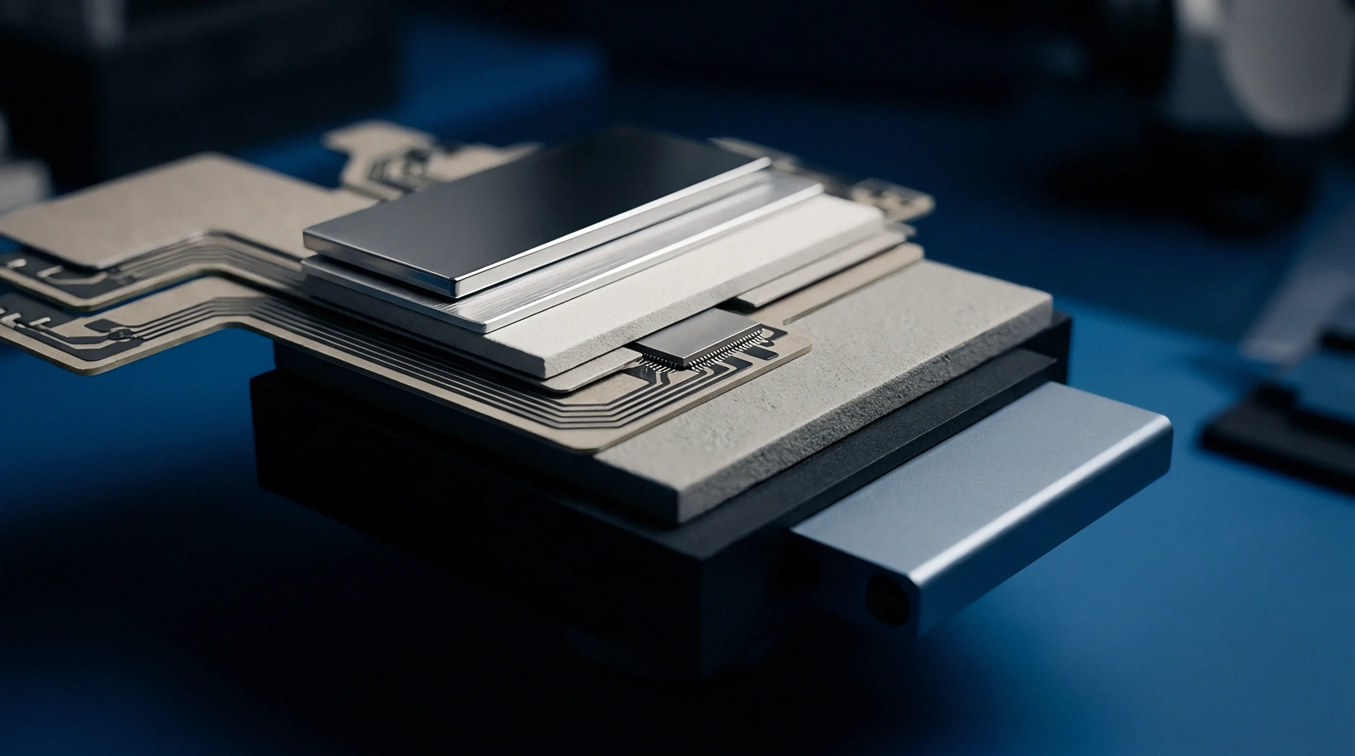
Sub-system performance acceptance specifications often define stage settling times using coarse positional tolerance windows. A motion stage vendor certifying axis positioning within a 1-micrometer band may still deliver high-frequency velocity jitter within that band. When the vision integrator mounts a high-magnification optical payload to that stage, angular deflection converts micro-scale translational stage jitter into sub-pixel image degradation, leading directly to rejected production batches and uncompensated redesign cycles.

Distortion
Optomechanical misalignment and thermal gradients skew wave-front geometry across custom imaging pathways. Optical errors within semi-custom vision payloads stem from manufacturing manufacturing tolerances, lens element assembly tilt, and thermal expansion of lens barrels. While static optical distortion can be calibrated using target grid matrices, dynamic optical distortion shifts non-linearly under changing operational temperatures and mechanical acceleration profiles.
Lens decentration destroys edge sharpness. Thermal expansion shifts the optical waist. Boresight tilt skews coordinate transform grids.
Chromatic dispersion broadens chromatic fringe zones. Element tilt degrades corner field resolution.
Optomechanical barrel construction dictates lens element position stability under physical acceleration. Custom vision applications frequently house multi-element glass groups inside aluminum, brass, or titanium barrels. Aluminum carries a thermal expansion coefficient of 23 parts per million per Kelvin, whereas optical glass ranges between 5 and 8 parts per million per Kelvin.
As internal lens barrel temperatures rise due to surrounding system electronics, differential thermal expansion alters air-space distances between optical elements, shifting the effective focal length and driving severe focal plane defocus.
A thermal gradient across an uncompensated aluminum lens barrel shifts the focal plane faster than passive depth of field can absorb.
How Does Optomechanical Thermal Expansion Shift Focal Planes?
Focal drift resulting from ambient and internal heat generation alters image plane location along the z-axis. High-resolution machine vision optics operating at large numerical apertures possess narrow depths of field, often under 15 micrometers. An internal lens barrel temperature increase of 10 Kelvin expands a 50-millimeter aluminum housing by 11.5 micrometers, shifting the primary focal plane entirely outside the physical sensor plane window.
This z-axis focal displacement reduces image contrast across all field locations equally, mimicking motion blur while originating entirely within passive optomechanical structures.
Off-axis mechanical acceleration loads deform lens element positioning rings. During 3g stage acceleration profile maneuvers, cantilevered optical elements tilt within their retainers if pre-load torques fall below mechanical threshold limits. Element tilt breaks rotational symmetry across the optical path, generating field-asymmetric astigmatism and variable corner defocus.
Calibration routines assuming fixed radial distortion models fail when mechanical loads dynamically distort barrel alignment during high-speed moves.
Field Aberrations and Mechanical Deflection
Optical barrel deformation alters wave-front phase distribution across the image field. Evaluating wave-front distortions requires separating static optical aberrations, such as spherical aberration or coma inherent to design prescriptions, from dynamic optomechanical deflections caused by structural stress. When a heavy optical lens assembly bolts to a moving stage carriage using uneven bolt torque sequences, internal mechanical stress transfers through the housing, deforming precision-ground optical element seats.
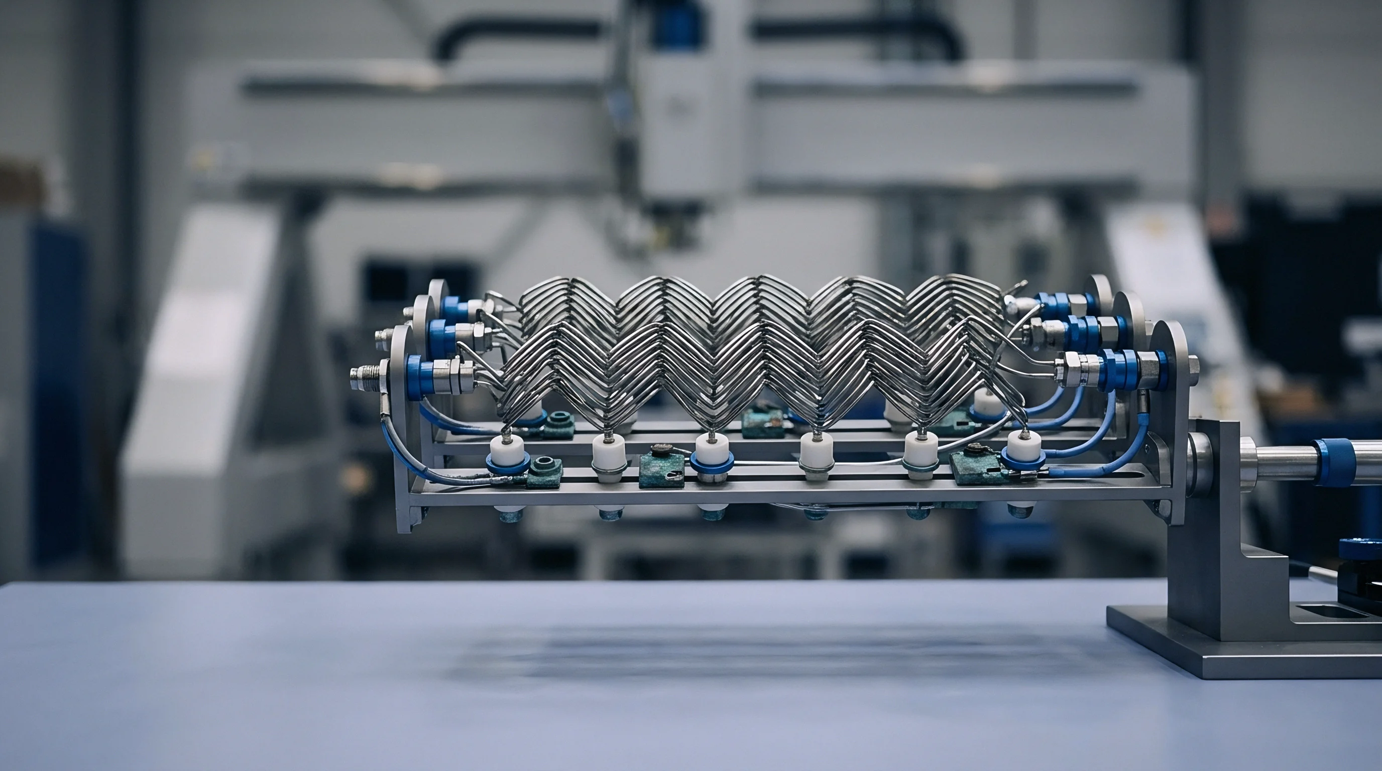
Off-the-shelf optical sub-assemblies carry nominal Modulation Transfer Function curves measured under ideal bench conditions. Optical suppliers baseline performance using collimated monochromatic light sources, rigid target mounts, and controlled 20-degree Celsius laboratory environments. In semi-custom integration, real-world mounting stresses, broad-spectrum LED lighting, and elevated operating enclosure temperatures degrade nominal optical performance significantly below published data sheet baselines.
The optics vendor claims the system met off-the-shelf MTF curves on an optical bench with monochromatic collimated lighting.
Coupling
Thermal dissipation and mechanical vibration interact across physical interfaces to compound total system error. Vision system failures rarely trace back to a single isolated component defect. Optical defocus, structural thermal expansion, and motion drive dynamics form coupled feedback loops where energy output from drive electronics drives mechanical degradation in adjacent vision sub-assemblies.
Linear motion drive motors generate considerable waste heat during high-frequency start-stop raster movement profiles. Continuous acceleration cycles drive stator temperatures up to 80 degrees Celsius. Thermal energy transfers via conductive paths through the stage mounting carriage directly into the camera support housing, heating lens elements and sensor chassis structures.
Simultaneously, mechanical acceleration forces excite bending resonance modes in cantilevered camera brackets, dynamically altering optical axis alignment relative to the target plane.
Failure to isolate motion drive heat sinks under ISO 10360 thermal drift guidelines voids sub-micron optical registration warranties.
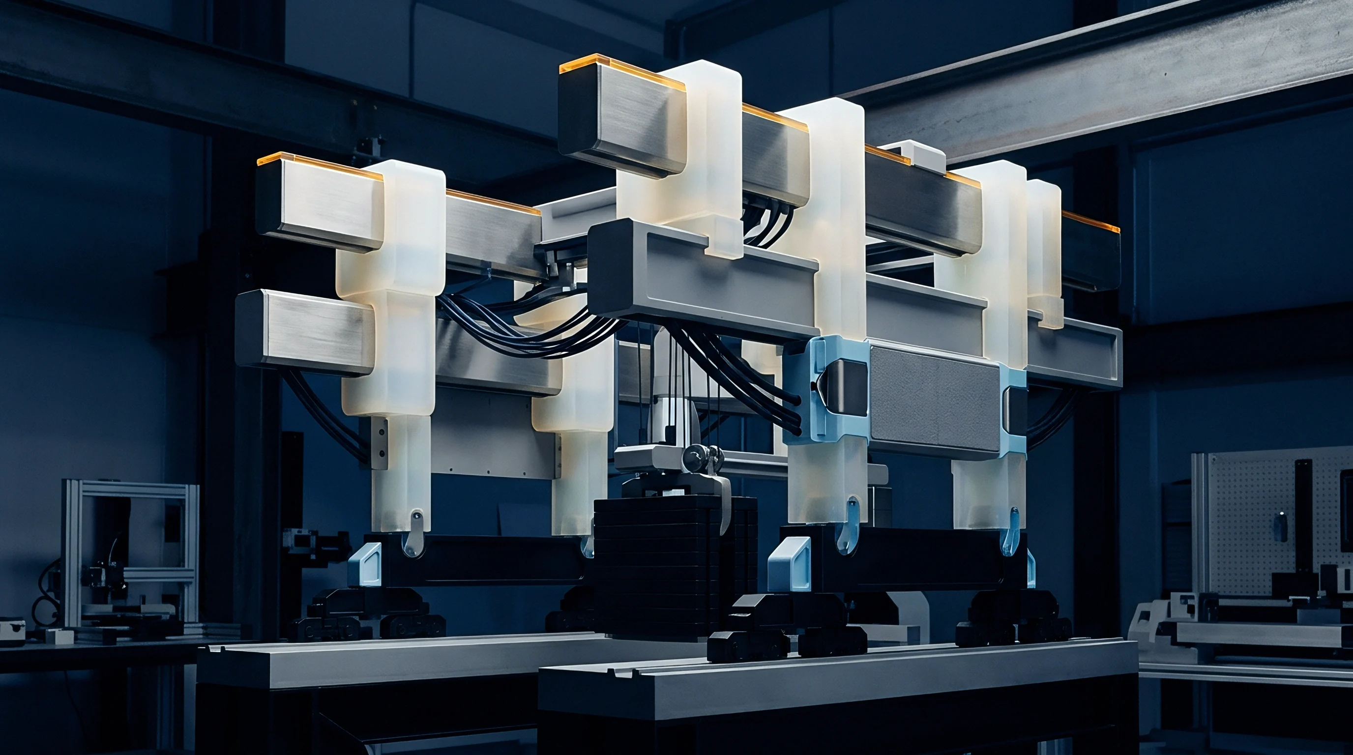
Optomechanical Thermal Interaction Mechanics
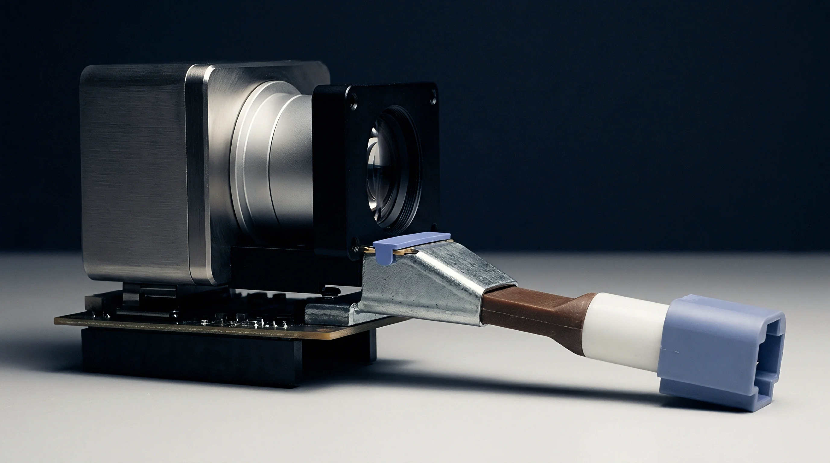
Quantifying multi-variable error coupling demands analyzing combined optical and motion error equations. Consider a semi-custom vision payload designed for automated wafer inspection, operating with a 5x optical magnification lens on a high-speed linear motor stage. The image sensor features a 3.45-micrometer pixel pitch, yielding a nominal object-space pixel size of 0.69 micrometers.
System performance contracts dictate sub-pixel feature registration accuracy within 0.35 micrometers.
During operation, linear motor stators dissipate 80 Watts of heat, elevating mounting plate temperatures by 18 Kelvin over 45 minutes of continuous operation. Conductive heat transfer through the camera bracket raises the lens barrel temperature by 12 Kelvin, causing an optomechanical z-axis focal expansion of 13.8 micrometers. Concurrently, high-speed motor stage directional reversals generate 2.5g acceleration impulses, exciting a 140 Hz mechanical bending mode in the camera mounting bracket that yields a peak angular deflection of 0.08 milliradians.
Focus displacement of 13.8 micrometers on a lens with a 12-micrometer depth of field degrades baseline static Modulation Transfer Function at 100 line-pairs per millimeter from 0.52 down to 0.18, broadening the optical point spread function diameter from 1.2 micrometers to 3.8 micrometers. Simultaneously, the 0.08-milliradian angular deflection across a 150-millimeter working distance creates a dynamic spatial displacement of 12 micrometers at the image target plane. Combined using root sum square spatial convolution, total effective spot uncertainty expands to 12.5 micrometers at the object plane, exceeding the 0.35-micrometer spatial registration budget by more than 35 times.
Temporal Trigger Timing and Sensor Readout Interactions
Rolling shutter CMOS image sensors read out image rows sequentially over a finite frame readout period. When periodic mechanical vibration interacts with sequential row exposure timing, straight spatial features appear distorted with spatial ripple artifacts. Line-scan vision payloads exhibit similar spatial distortion patterns when encoder pulse trigger rates fluctuate due to mechanical velocity jitter.
Encoder trigger timing jitter distorts line-scan image geometry along the motion axis. If stage motion velocity drops momentarily while line-scan trigger frequencies remain fixed, the sensor samples the same physical area multiple times, artificially stretching feature dimensions along the motion axis. Conversely, stage velocity spikes cause skipped spatial intervals, compressing feature geometry.
When optical defocus simultaneously blurs feature edge boundaries, automated defect classification software cannot distinguish between physical part defects, optical defocus blur, or encoder trigger timing errors.
Mounting high-dissipation motor drives directly to optical support structures guarantees unresolvable spatial calibration drift.
Isolation
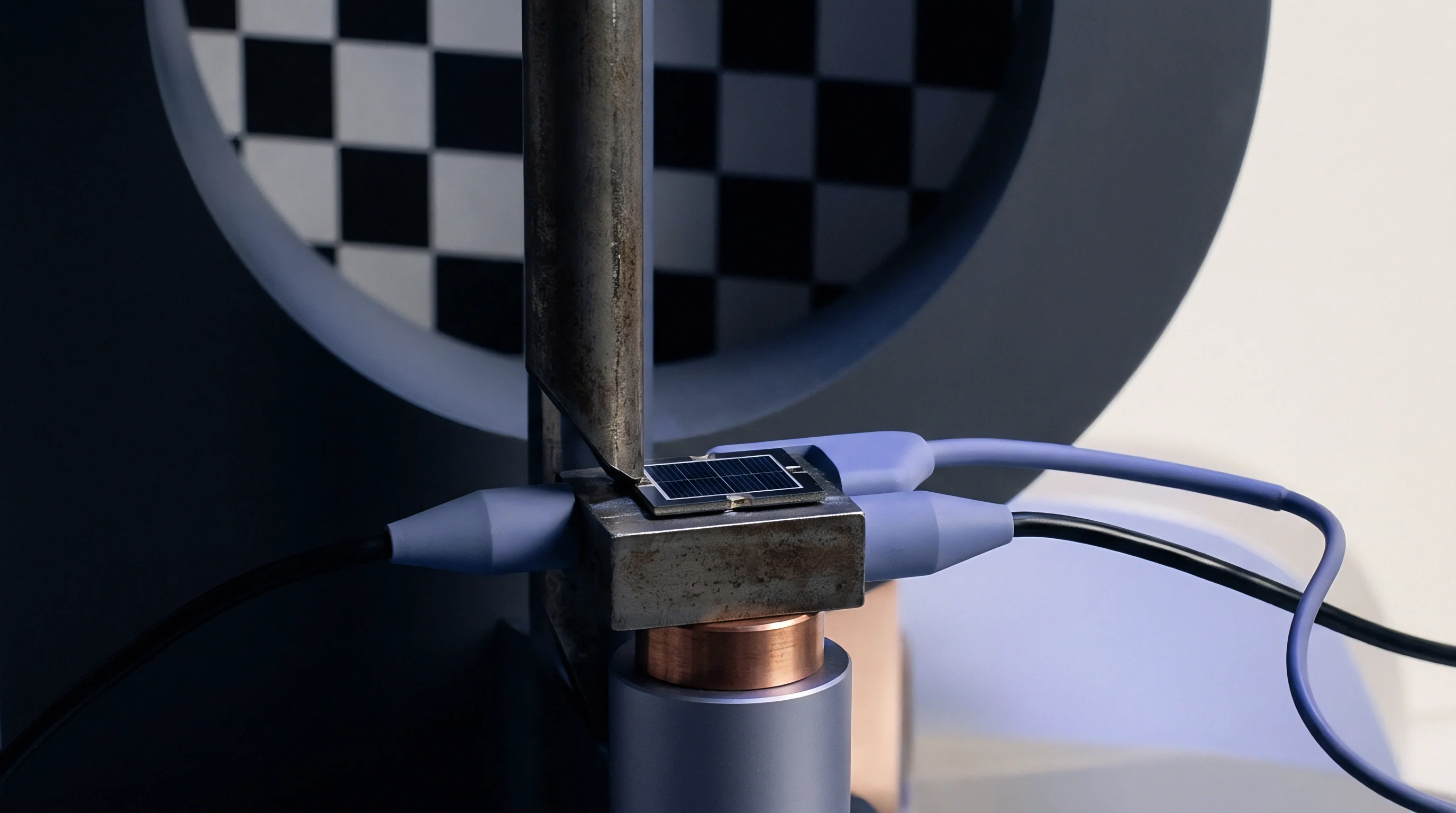
Experimental test benches separate dynamic mechanical noise from static optical wavefront degradation. Attributing field failure root causes between optical sub-assembly defects and motion stage instability requires empirical isolation techniques. Testing vision payloads in fully assembled operational configurations masks root cause contributions because optical defocus and motion blur produce overlapping spatial intensity degradation signatures.
Stroboscopic flash freezes motion blur. Interferometers track real time axis displacement. Static targets isolate pure optical field tilt.
Decoupled test fixtures isolate vibration sources.
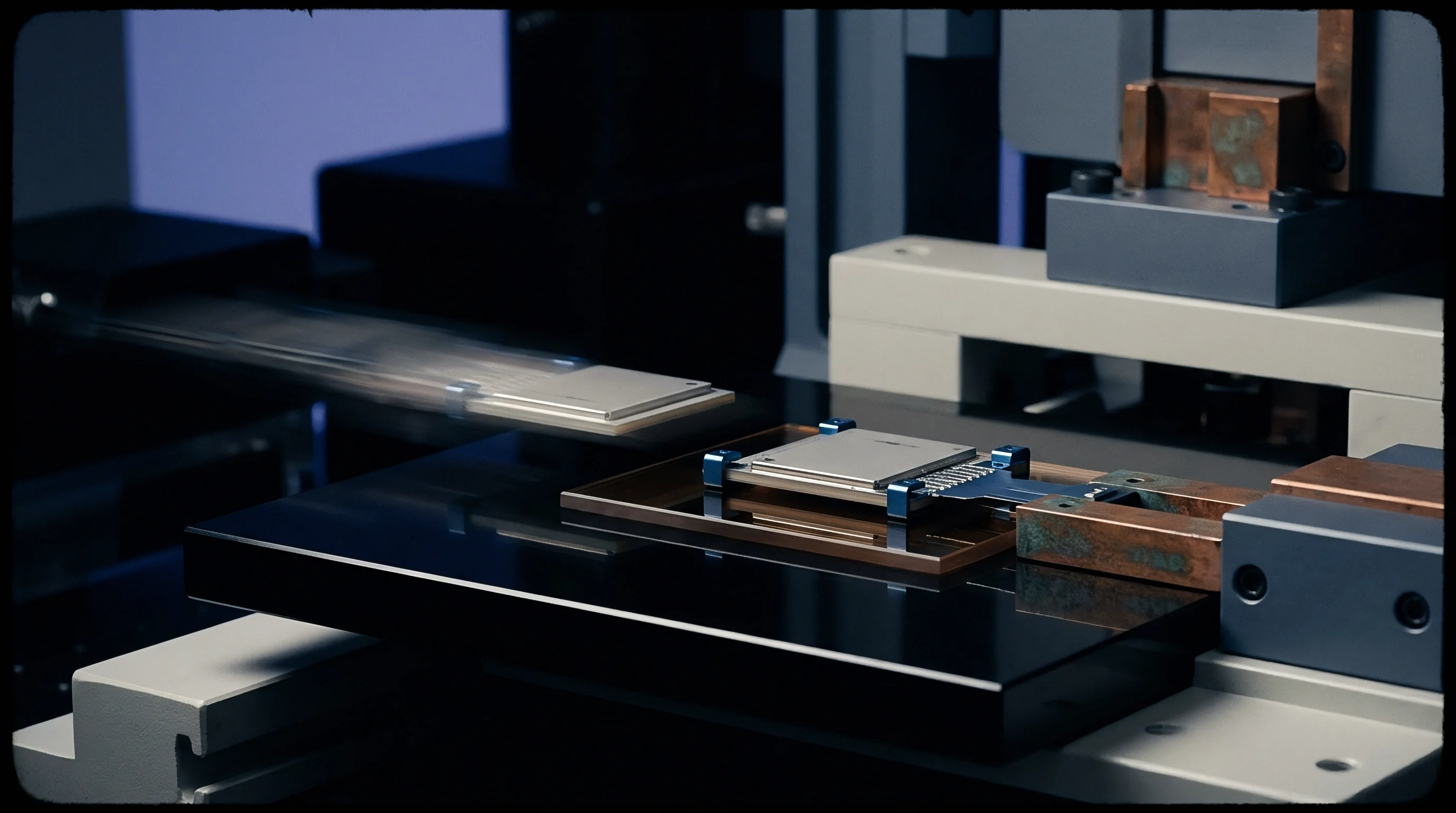
Separating optical aberrations from motion disturbances relies on manipulating temporal exposure windows and physical illumination modes. Replacing continuous illumination sources with ultra-short pulsed LED or laser illumination suppresses the motion exposure window (texp) to sub-microsecond levels. Pulsed illumination reduces motion blur to near zero regardless of stage velocity, allowing engineers to evaluate pure optical Modulation Transfer Function under active operational stage speeds.
Stroboscopic pulse widths below two hundred nanoseconds eliminate linear motion blur for stage velocities up to five hundred millimeters per second.
Step by Step Diagnostic Isolation Method
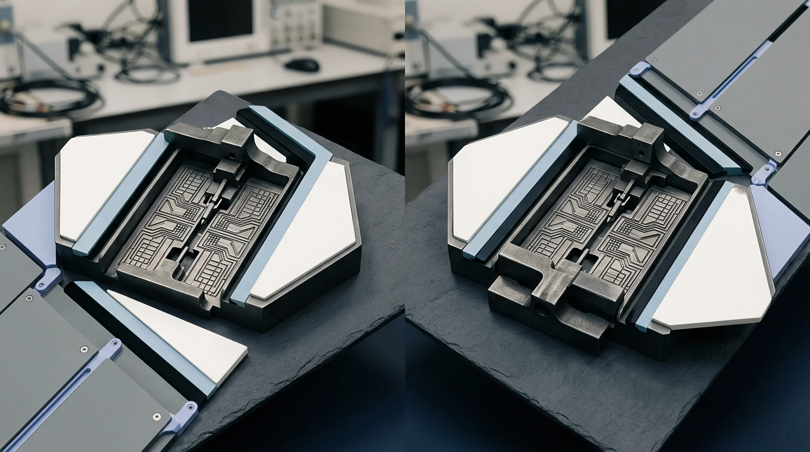
Isolating optical defocus from mechanical motion jitter uses a structured physical test sequence on an optical isolation table.
- Mount the entire optical camera sub-assembly onto an isolated granite optical bench completely uncoupled from the motion stage structure.
- Position a illuminated glass calibration target on the moving axis stage and record static optical resolution baselines across the field of view.
- Execute full operational speed motion profiles while illuminating the target with stroboscopic pulses under two hundred nanoseconds duration to capture pure optical performance under vibration.
- Switch illumination to continuous operational mode with standard exposure settings to capture combined optomechanical performance data.
- Subtract the stroboscopic optical image dataset from the continuous exposure dataset to isolate the pure mechanical motion blur point spread function matrix.
- Attach non-contact laser Doppler vibrometer sensors to the lens housing, sensor flange, and stage carriage to map high-frequency mechanical transfer functions across all axes.

Diagnostic Equipment and Parameter Decoupling
Determining root cause allocations across sub-assembly interfaces demands specialized metrology equipment and structured test conditions. The testing matrix matches diagnostic instrumentation against specific error mechanisms to ensure unambiguous data collection.
| Test Configuration | Diagnostic Instrument | Target Measured Parameter | Segregation Confidence Level |
|---|---|---|---|
| Stroboscopic Target Capture | Sub-microsecond LED Strobe | Pure Optical MTF under Dynamic Load | High (>95% Motion Blur Suppression) |
| Non-Contact Structural Tracking | Laser Doppler Vibrometer | Camera Housing Angular Deflection | High (>98% Amplitude Accuracy) |
| Thermal Field Mapping | Infrared Thermography Camera | Motor-to-Optics Conductive Gradient | Medium (Surface Temperature Only) |
| Encoder Timing Correlation | High-Speed Logic Analyzer | Line-Trigger Synchronization Jitter | High (<10 ns Time Resolution) |
Correlating spatial image edge degradation against real-time laser Doppler vibrometer vibration spectra allows engineers to attribute specific spatial blur artifacts to distinct mechanical resonance frequencies. When a 220 Hz vibration spike logged on the optical barrel matches a 220 Hz spatial frequency ripple across captured image edge profiles, motion stage structural compliance stands proven as the primary error contributor.
Whether high-frequency structural resonances measured at the mounting flange remain linear when temperature shifts mechanical damping ratios stays an open empirical question.
Apportionment
Statistical error budgets assign quantitative measurement bounds across sub-assembly scope lines. Once test protocols isolate optical and motion error contributions, system integrators must assign mathematical variance weights to establish formal supplier accountability limits. Combining multi-variable error terms into unified analytical budgets prevents commercial disputes over warranty liability during volume manufacturing ramp phases.
Variance summation defines total system uncertainty. Thermal cross-covariance expands error bounds. Clear scope lines prevent warranty disputes.
Root sum square math models independent errors.
Traditional error budgeting relies on Root Sum Square summation models assuming independent, uncorrelated gaussian error distributions. In semi-custom vision systems, mechanical acceleration profiles, heat generation, and optomechanical deflections exhibit strong cross-covariance, rendering simple RSS models overly optimistic. Advanced error allocation models incorporate cross-covariance matrix terms to account for thermal and mechanical interactions between sub-assemblies.
Unallocated error terms in an optomechanical specification sheet inevitably end up billed to the party managing final system integration.
Variance Allocation Formula and Covariance Structuring
Mathematical root cause apportionment calculates total image spatial uncertainty (σtotal2) by summing individual sub-system variance vectors along with their mutual cross-covariance terms across defined operating conditions:
σtotal2 = σoptics2 + σmotion2 + σthermal2 + σsensor2 + 2· Cov(optics, thermal) + 2· Cov(motion, dynamic)
Evaluating this statistical model requires populating each variance term using empirical metrology data gathered during diagnostic isolation phases. The covariance term Cov(optics, thermal) captures lens barrel focal shift caused by motor heat dissipation, while Cov(motion, dynamic) models camera mounting bracket angular deflection under stage acceleration impulses. Neglecting cross-covariance terms leads integrators to underestimate total spatial registration drift by up to 50 percent in continuous operational environments.
Commercial Interface Definition and Scope Transfer
Translating mathematical error allocations into enforceable commercial supply contracts demands clear technical interface parameters. When buying semi-custom vision sub-assemblies, technical procurement contracts must define exact boundary test conditions under which each vendor must demonstrate compliance.
- Optical baseline acceptance criteria define minimum spatial Modulation Transfer Function thresholds measured across five field locations under standardized stroboscopic lighting conditions on rigid test benches.
- Motion stage dynamic tolerance boundaries specify maximum allowable velocity jitter bands and settling time limits under defined payload mass and acceleration profiles.
- Thermal interface boundary conditions constrain heat flux limits transmitted across mechanical mounting surfaces connecting drive motors to camera support structures.
- Firmware trigger timing jitter thresholds limit allowable time latency variations between motion encoder position pulses and camera frame-grabber trigger input pins.
Defining clear technical scope lines on design transfer packages establishes objective acceptance parameters before volume tooling expenditures occur. When an integrated vision system fails final factory acceptance testing, non-recurring engineering costs and rework expenses land on the vendor whose sub-assembly exceeded its allocated variance budget line under agreed test conditions.
| Error Component | Sub-System Source | Allocation Budget | Measurement Standard | Responsible Party Scope |
|---|---|---|---|---|
| Static Wavefront Aberration | Lens Optomechanics | < 0.15 Pixels MTF Drop | ISO 12233 Stroboscopic Test | Optics Sub-Assembly Supplier |
| Dynamic Boresight Tilt | Camera Mounting Bracket | < 0.02 mrad Deflection | Laser Doppler Vibrometry | Mechanical Frame Fabricator |
| High-Frequency Axis Jitter | Linear Drive and Encoder | < 0.25 µm Displacement | ISO 230-2 Motion Calibration | Motion Stage Manufacturer |
| Thermal Focal Drift | Motor Heat Dissipation | < 3.0 µm Focus Shift | ISO 10360 Thermal Test | System Integration Engineer |
Inserting ISO 230-2 motion accuracy compliance clauses alongside ISO 12233 optical resolution limits into the master scope contract binds component suppliers to independent acceptance testing prior to final payload assembly.