Matching Network Topologies for Embedded Transceiver Integration
Embedded transceiver matching network topologies require impedance conjugate translation, parasitic pad cancellation, substrate verification, and contractual design transfer.
Mismatch
Silicon transceivers present complex source and load impedances that deviate significantly from standard fifty-ohm system traces. Modern sub-gigahertz, 2.4 GHz, and 5.8 GHz transceiver integrated circuits output differential or single-ended port impedances such as 15 + j28 ohms or 35 – j12 ohms depending on the internal power amplifier output stage and low-noise amplifier input configuration. Matching networks translate these complex silicon impedances into standard transmission line impedances to prevent power reflections, maximize power transfer, and optimize receiver noise figures.
Direct traces without reactive matching elements degrade return loss and risk violating harmonic radiation limits.
Complex Conjugate Target Definitions
Radio frequency power amplifier outputs require exact load transformation to maximize RF power delivery to the antenna. The ideal load impedance equals the complex conjugate of the transceiver output impedance. When a transmitter RF pin presents an internal output impedance of 20 + j35 ohms, the matching network input must present 20 – j35 ohms to extract maximum output power.
Realizing this target requires precise reactive elements placed directly adjacent to the transceiver output pads. Incorrect match selection increases internal thermal dissipation on silicon, dropping transmit power efficiency by two to four decibels and raising junction temperatures.
| Frequency Band | Chipset Port Type | Silicon Source Impedance | Target Load Impedance | Balun Requirement | Typical Insertion Loss |
|---|---|---|---|---|---|
| 433 MHz / 915 MHz | Differential Open-Drain | 12 + j22 ohms | 12 – j22 ohms | External Discrete Balun | 0.4 dB to 0.7 dB |
| 2.4 GHz ISM | Differential Matched | 30 + j40 ohms | 30 – j40 ohms | Integrated Ceramic IPD | 0.8 dB to 1.2 dB |
| 5.8 GHz ISM | Single-Ended 50-Ohm | 42 – j8 ohms | 42 + j8 ohms | None (Direct Transmission) | 0.3 dB to 0.5 dB |
| 2.4 GHz / 5 GHz Dual | Differential High-Z | 15 – j60 ohms | 15 + j60 ohms | LTCC Front-End Module | 1.1 dB to 1.6 dB |

Differential Transceiver Interface Synthesis
Balanced port outputs reduce common-mode noise while generating harmonic spurs that demand symmetrical passive filtering. Differential matching structures combine matching reactive branches with balance-to-unbalance conversion elements, commonly termed baluns. Integrated circuit vendors often mandate discrete lattice baluns or low-temperature co-fired ceramic components to transition differential signals to single-ended antenna lines.
Lattice baluns utilize two low-pass and two high-pass paths configured in a bridge to achieve a 180-degree phase shift between output legs. Symmetrical component placement is mandatory; asymmetry introduces phase imbalance, converting differential RF power into common-mode currents that radiate directly from ground planes and violate electromagnetic compatibility standards.
At 2.4 GHz, a 1.0 nH inductance variation in a high-Q series arm shifts return loss by 8.5 dB across a 50-ohm interface.
Receiver performance relies equally on input impedance transformation. Low-noise amplifier inputs require a match optimized for minimum noise figure rather than maximum power transfer. The optimum noise source impedance (Zopt) rarely equals the complex conjugate of the input impedance (Zin ).
Designing an input network requires balancing return loss against noise figure degradation. A matching network optimized strictly for power transfer can degrade receiver sensitivity by 1.5 dB to 3.0 dB, reducing line-of-sight communication range by up to thirty percent.
Selecting incorrect load targets causes power amplifier distortion, degrades transmitter efficiency, reduces battery operating lifetime, and increases engineering costs during compliance testing.


Coil
Discrete surface-mount inductors provide the reactive energy storage necessary to cancel capacitive chip impedance. Wire-wound and multilayer ceramic inductors exhibit vastly different high-frequency characteristics that impact RF signal path performance. Wire-wound inductors offer higher quality factors (Q) ranging from 30 to 80 at 2.4 GHz, minimizing resistive insertion loss across matching branches.
Multilayer ceramic inductors provide lower cost and tighter dimensional control but exhibit Q factors between 10 and 25. Choosing lower Q passives introduces thermal dissipation within the matching network itself, lowering transmitted output power.
Inductor Quality Factor Restrictions
Component loss tangent dictates the total insertion dissipation across passive matching branches. A low-Q matching inductor converts transmit energy into heat. In battery-powered IoT nodes, a 0.5 dB loss in the RF front-end equates to a twelve percent drop in operational battery life.
Wire-wound components reduce resistive losses but occupy larger surface mount footprints. Multilayer components reduce PCBA area while increasing signal attenuation. High-Q series inductors widen matching bandwidth while steepening out-of-band rejection curves in harmonic filtering networks.
Self-Resonant Frequency Thresholds
Internal winding capacitance alters component behavior beyond specific operational frequency limits. Every discrete inductor carries parasitic inter-turn capacitance that forms a parallel resonant circuit with its nominal inductance. At the self-resonant frequency, the component impedance approaches infinity before turning purely capacitive at higher frequencies.
RF matching networks must utilize inductors with self-resonant frequencies at least two to three times higher than the transceiver operating frequency. An inductor operating near its self-resonant frequency suffers from extreme inductance value drift caused by slight temperature shifts.
- Self-Resonance Saturation Component reactive impedance turns capacitive above the self-resonant frequency, destroying the intended matching phase angle.
- Mutual Inductive Coupling Unshielded magnetic fields interact with neighboring trace loops, introducing unintended crosstalk across receiver paths.
- Dielectric Thermal Drift Substrate expansion under power amplifier heat alters passive physical geometries, shifting tuning targets.
- Solder Fillet Parasitics Excessive solder deposition adds stray capacitance between terminal pads and internal ground planes.
Physical placement of discrete inductors dictates coupling levels across adjacent RF paths. Unshielded surface-mount inductors leak magnetic flux, inducing unwanted voltages into adjacent PCB traces. Laying out two series inductors parallel to one another creates mutual inductive coupling, modifying effective inductance values by fifteen to twenty-five percent.
Rotating adjacent inductors ninety degrees relative to each other eliminates mutual flux linkage, securing target filter poles.
Orienting adjacent surface-mount inductors at right angles minimizes mutual magnetic coupling across compact printed circuit layouts.
Substrate
Printed circuit board dielectric layers dictate transmission line characteristic impedance and signal velocity. Standard FR-4 laminates consist of woven fiberglass cloth impregnated with epoxy resin. The ratio of glass cloth to resin varies across manufacturing lots, causing the relative dielectric constant (varεr) to fluctuate between 3.8 and 4.8 at 2.4 GHz.
High-frequency designs using FR-4 experience impedance shifts along microstrip traces. Hydrocarbon ceramic laminates like Rogers 4003C offer a controlled dielectric constant of 3.38 ± 0.05, maintaining tight microstrip line width calculations.
Dielectric Constant Variations across Manufacturing Runs
Laminate manufacturers permit thickness and glass-to-resin ratio tolerances that alter trace capacitance. Standard commercial PCB fabricators quote dielectric thickness tolerances of ± 10%. On a four-layer stackup with a 0.175 mm outer dielectric layer, a ten percent thickness variation alters fifty-ohm microstrip trace impedance by approximately 4.2 ohms.
This impedance variation shifts matching network pole locations, increasing RF return loss from a nominal -25 dB to -12 dB. Substrate loss tangent (tan δ) also drives signal dissipation; standard FR-4 dissipates 0.02 at 2.4 GHz, whereas low-loss RF laminates exhibit dissipation factors below 0.0027.
| Substrate Material | Dielectric Constant (varεr at 2.4 GHz) | Dissipation Factor (tan δ) | Copper Roughness (Rz) | Impedance Shift per 10 $mu$m Trace Error |
|---|---|---|---|---|
| Standard FR-4 (370HR) | 4.50 ± 0.35 | 0.0200 | 6.0 $mu$m | ± 3.8 ohms |
| High-Tg FR-4 | 4.20 ± 0.20 | 0.0150 | 4.5 $mu$m | ± 2.9 ohms |
| Rogers RO4003C | 3.38 ± 0.05 | 0.0027 | 2.1 $mu$m | ± 1.1 ohms |
| Polyimide Flex | 3.20 ± 0.15 | 0.0050 | 1.5 $mu$m | ± 1.6 ohms |
Coplanar Waveguide Ground Clearance Rules
Ground plane spacing beside RF signal lines controls electric field distribution and effective permittivity. Conductor-backed coplanar waveguides utilize top-layer ground pours separated from signal microstrips by a specified gap (g). Narrowing the ground gap increases ground capacitance per unit length, lowering characteristic impedance.
Standard design rules dictate maintaining a ground gap at least 1.5 times the trace width to prevent excessive electric field concentration in the solder mask layer. Liquid photo-imageable solder mask materials exhibit unstable dielectric constants between 3.5 and 4.2, introducing unexpected attenuation when allowed to flow into high-field microstrip regions.
IPC-TM-650 Method 2.5.5.5 mandates permittivity testing at 10 GHz, penalizing fabricators who measure substrate dielectric constants at lower audio frequencies.
Copper surface roughness contributes measurable attenuation at microwave frequencies due to skin effect skin-depth limitations. At 5.8 GHz, copper skin depth equals approximately 0.85 micrometers. Standard electrodeposited copper foils present surface roughness (Rz) values between 5 and 9 micrometers.
When surface profile peak-to-valley dimensions exceed skin depth, RF currents follow the physical contours of the copper peaks, increasing effective path length and conductor resistance. Specifying reverse-treated or low-profile copper foils ($R_z
Raw laminate permittivity variations can remain within standard commercial specifications even when trace impedance shifts push transceiver harmonic emissions past statutory limits.


Topology
Matching network component configurations determine transformation bandwidth, harmonic suppression depth, and insertion loss figures. Designers evaluate three core discrete structures: L-networks, Pi-networks, and Tee-networks. L-networks consist of two reactive elements offering a single fixed quality factor set strictly by the ratio of source to load resistance (Q = sqrtRhigh / Rlow – 1).
Pi-networks and Tee-networks incorporate three reactive elements, granting independent control over system operating bandwidth and transformation ratio. Selection depends on target harmonic attenuation requirements and layout board area constraints.

Pi Network Harmonic Filtering
Dual shunt capacitors paired with a series inductor form a low-pass structure that suppresses high-order transmitter harmonics. Transceiver power amplifiers generate unwanted power at second and third harmonic frequencies. A properly synthesized Pi-network transforms complex silicon impedance to 50 ohms while simultaneously providing 25 to 40 dB of attenuation at the second harmonic frequency.
Shunt capacitors absorb stray parasitic capacitance contributed by transceiver bond wires and PCB surface pads, which would otherwise degrade return loss.
| Topology Type | Element Count | Insertion Loss at 2.4 GHz | 2nd Harmonic Attenuation | Transformation Bandwidth | Substrate Footprint |
|---|---|---|---|---|---|
| Series L / Shunt C (L-Net) | 2 | 0.2 dB to 0.4 dB | 8 dB to 12 dB | Fixed (Narrowband) | 2.1 mm2 |
| Shunt C / Series L / Shunt C (Pi) | 3 | 0.5 dB to 0.8 dB | 28 dB to 38 dB | Flexible (Broadband) | 3.8 mm2 |
| Series L / Shunt C / Series L (Tee) | 3 | 0.6 dB to 0.9 dB | 18 dB to 24 dB | Flexible (High-Z Source) | 4.2 mm2 |
| Integrated Passive Device (IPD) | Monolithic | 0.7 dB to 1.1 dB | 35 dB to 45 dB | Pre-tuned (Fixed Band) | 1.2 mm2 |
Tee Topologies for High Source Impedance Transformation
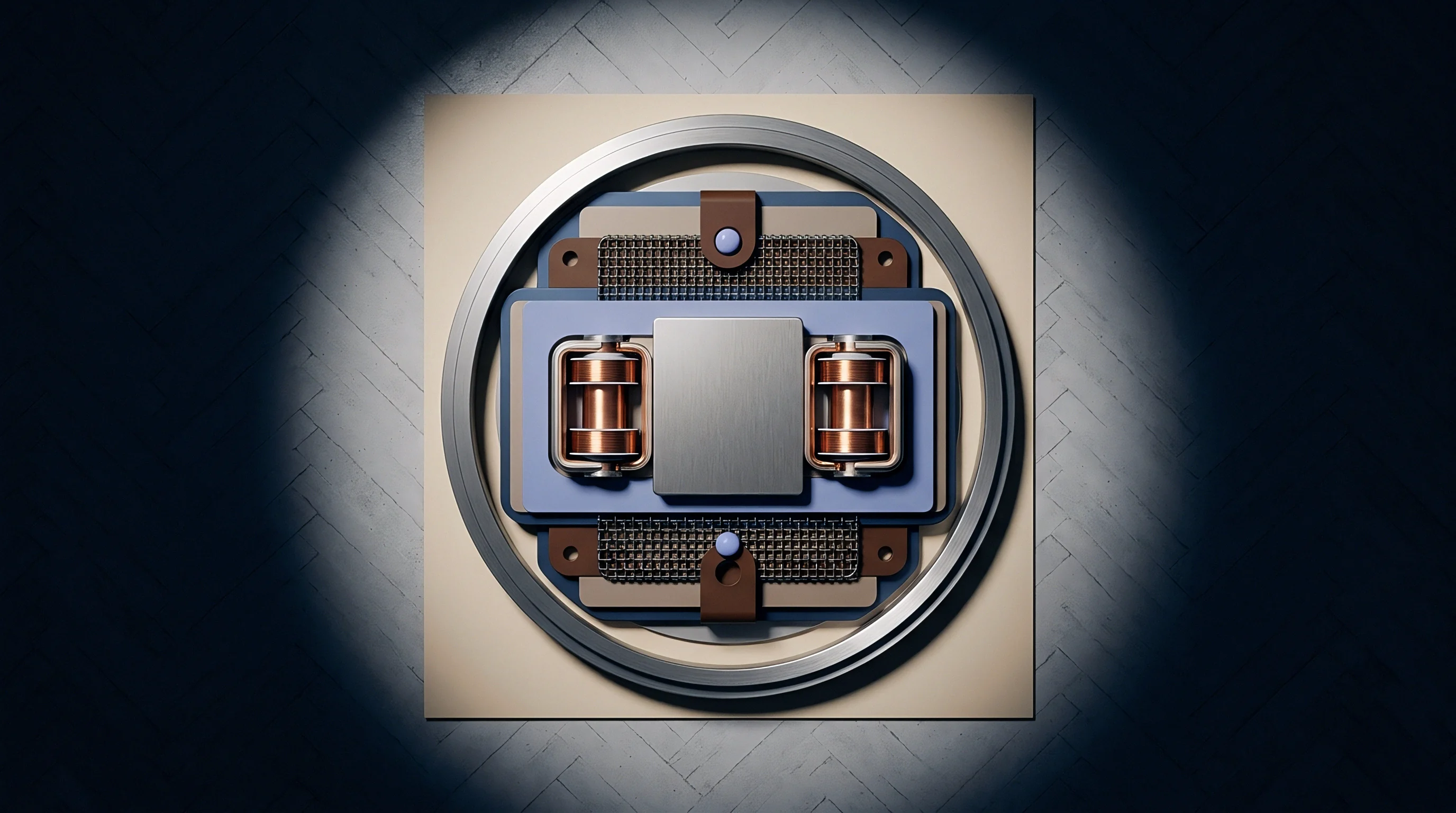
Series inductive arms combined with a single shunt capacitor convert high source resistance down to standard system levels. Tee-networks perform effectively when matched to highly capacitive transceiver ports. Placing a series inductor directly at the transceiver output cancels internal chip pad capacitance, allowing the subsequent shunt capacitor and series inductor to match real resistive loads smoothly.
Tee structures occupy slightly larger board areas due to the physical footprint of two discrete inductors. Inductor spatial orientation demands careful layout to prevent mutual coupling between the input and output arms.
- Calibrate vector network analyzer port cables using full two-port short-open-load-thru calibration standards.
- Measure unpopulated circuit board pad complex impedance across the operational frequency band.
- Calculate initial L-network series and shunt passive values using Smith chart transformation equations.
- Solder selected high-Q components onto circuit board pads using controlled thermal profiles.
- Adjust discrete component values iteratively to neutralize parasitic pad capacitance and trace inductance.
Mathematical derivation of an L-network matching circuit requires calculating reactance values based on load and source resistances. Consider a 2.4 GHz transceiver presenting a single-ended output impedance of ZS = 15 – j30 Ω that must match a ZL = 50 Ω antenna. The matching network must first cancel the -j30 Ω capacitive reactance with a +j30 Ω series inductance component.
Next, the real 15 Ω source resistance must be stepped up to 50 Ω. The required node quality factor QN is calculated as:
QN = sqrtfrac5015 – 1 = sqrt3.333 – 1 = sqrt2.333 ≈ 1.527
The parallel capacitive reactance XP required across the 50 Ω load is calculated by dividing the load resistance by the node quality factor:
XP = frac501.527 ≈ 32.74 Ω
Converting this capacitive reactance to a physical capacitance at 2.4 GHz yields:
Cshunt = frac12 π × 2.4 × 109 × 32.74 ≈ 2.02 pF
The series reactive arm must supply both the transformation inductance XStrans = QN × 15 = 1.527 × 15 = 22.91 Ω and the +j30 Ω chip pad cancellation reactance. Summing these reactances gives a total series inductive reactance of XStotal = 22.91 + 30 = 52.91 Ω. Converting this total reactance to a physical inductance at 2.4 GHz yields:
Lseries = frac52.912 π × 2.4 × 109 ≈ 3.51 nH
Assuming a standard 0402 surface-mount capacitor tolerance of ± 0.1 pF and an inductor tolerance of ± 2%, actual physical implementation defaults to commercial values: a 2.0 pF capacitor and a 3.6 nH inductor, though lower quality factors will reduce selectivity.
RF design engineers select integrated passive devices when printed circuit board space constraints prevent placing six discrete surface-mount components within three millimeters of transceiver pins.


Tolerance
Component value variances combine with substrate manufacturing deviations to create random RF return loss distributions. Standard commercial surface-mount capacitors and inductors carry component value tolerances of ± 5%, ± 10%, or ± 0.1 pF. In narrowband matching topologies, a five percent inductance shift moves the center matching frequency by up to 60 MHz at 2.4 GHz.
High-volume manufacturing lines require statistical tolerance modeling to guarantee target yield percentages without individual manual bench tuning.
Monte Carlo Yield Predictions
Statistical circuit simulations evaluate thousands of component value permutations to calculate production pass rates. Running a 1,000-run Monte Carlo trial applies Gaussian distribution curves across passive component tolerances, PCB trace width variations, and substrate dielectric constant drift. The resulting yield histogram shows the probability of achieving a return loss better than -15 dB across the entire operating temperature range.
Designing networks with lower node quality factors ($Q_N

Can Discrete Passive Tolerances Override Stackup Deviations?
High-precision passive components with tight value bands compensate effectively for minor dielectric layer variations across manufacturing lots. Standard FR-4 permittivity shifts alter line impedance by several ohms, but specifying 1% wire-wound inductors and C0G ultra-tight capacitance passives limits matching network pole drift. Thermal coefficient ratings play a central role; C0G/NP0 ceramic capacitors exhibit zero temperature drift (± 30 p±/circC), whereas X7R materials drop capacitance by up to fifteen percent at operating temperatures above 85 degrees Celsius.
- Capacitor Dielectric Selection Specify C0G or NP0 ceramics to maintain stable capacitance across operational temperature ranges.
- Inductor Tolerance Banding Select one-percent or tight-tolerance wire-wound inductors for narrow-band matching branches.
- Thermal Drift Compensation Calculate passive value shifts caused by temperature coefficient expansion during continuous transmission.
- Reflow Solder Pad Symmetry Design symmetrical copper pads to eliminate component tombstoning and asymmetric parasitic pad capacitance during reflow.
Reflow thermal profiles alter passive values through component mechanical stress and solder volume variability. Thermal expansion during soldering forces tiny physical adjustments inside ceramic capacitor layers, shifting nominal baseline values by 0.5% to 1.5%. Solder paste volume repeatability dictates parasitic ground capacitance.
Automated optical inspection verifies physical component placement, but absolute RF performance verification requires automated end-of-line return loss sampling using calibrated network analyzers.
Selecting surface-mount passives with self-resonant frequencies far above the operating harmonic protects the receiver sensitivity from unwanted parasitic resonance.
RF integration teams continue to debate whether automated real-time tuner circuits integrated directly into silicon will eventually replace discrete board-level matching networks in sub-six gigahertz devices.


Handover
Design transfer documentation specifies the exact physical, electrical, and manufacturing deliverables transferred between engineering design houses and production facilities. A turnkey module contract transfers full design ownership, including Gerber stackups, schematic CAD files, bill of materials liability, and firmware RF register code. Semi-custom integration limits deliverables to pre-compiled binaries and reference layout snippets.
Engineering procurement teams demand clear deliverable dossiers to prevent commercial lock-in and enable dual-sourcing options.

Turnkey Module Scope Boundaries
Turnkey agreements place complete responsibility for RF regulatory certification and production yield on the module vendor. The vendor delivers fully tested printed circuit board assemblies carrying modular FCC/CE certifications. This path minimizes internal engineering headcount but increases per-unit production cost by 25% to 45%.
The buyer receives completed physical modules but lacks rights to modify trace geometries or swap underlying passive component suppliers without voiding vendor warranties.

Design File Transfer Formats
Complete design transfers demand unencrypted open-source native files rather than flattened static outputs. Sourcing specifications mandate native Altium Designer or KiCad project files containing complete netlists, padstack libraries, and copper balance rules. Gerber X2 or IPC-2581 outputs carry layer order definitions, material stackup specs, and embedded drill attributes directly to the PCB fabricator.
Omission of native CAD files restricts the buying team from altering matching network traces during subsequent product hardware iterations.
- Native CAD Schematics Transfer unencrypted project schematics including complete symbol libraries and netlist specifications.
- Gerber X2 Fabrication Dossier Provide Gerber X2 or IPC-2581 manufacturing files containing drill tables and copper layer definitions.
- RF Calibration Test Vectors Define vector network analyzer calibration procedures and acceptable return loss limits for end-of-line verification.
- Firmware Register Sequences Document transceiver initialization sequences and power amplifier bias setting registers in plain source code.
Firmware integration files control matching performance through internal register settings. Modern transceivers embed programmable internal tuning capacitors and adjustable power amplifier bias currents. Transfer packages must include low-level C source code drivers that write calibration registers during system startup.
Delivering compiled binary blobs leaves the buying organization vulnerable when driver updates break operating system compatibility or require register patches to resolve newly discovered silicon errata.
Semiconductor vendors supply reference layouts optimized for evaluation fixtures rather than space-constrained commercial enclosures.
Incorporating IPC-2581 Class 3 design transfer requirements into procurement contracts prevents contract manufacturers from substituting alternative RF passives without repeating return loss verification tests.