Quantifying RF Mismatch Degradation from Substrate Stackup Variance
Substrate dielectric tolerance and etch variance shift trace impedance, raising return loss and degrading RF power amplifier efficiency in custom module designs.

Glass
Woven reinforcing structures bound inside polymer dielectric matrices introduce localized shifts in permittivity across high-frequency layouts. Printed circuit board laminates depend on glass fiber fabric impregnated with resin to maintain structural rigidity and electrical insulation, but the underlying composite architecture is non-uniform. Glass fiber bundles carry a relative dielectric constant near 6.1, while common thermosetting epoxy, hydrocarbon, and PTFE resins sit between 2.1 and 3.8.
As an RF microstrip or stripline trace runs across the board, the effective dielectric constant seen by the wave fluctuates depending on whether the trace sits directly over a dense bundle or over a resin-filled gap, changing local capacitance and phase velocity along the path.
The scale of this dielectric variance is driven by the glass weave style specified in the fabrication drawing. Standard fabrics like style 7628 use heavy yarn with wide bundle spacing, producing dielectric constant shifts as large as plus or minus 0.40 over small distances. Medium weaves like 2116 tighten this gap, while spread-glass fabrics such as 1080, 1078, and 106 flatten and spread individual filaments across the plane.
These spread-glass structures pull localized dielectric variance down below plus or minus 0.05, stabilizing phase velocity and impedance down the line. Conductor routing relative to the weave axis plays a key role too: traces running strictly parallel or perpendicular to warp and weft yarns remain over continuous resin-rich or glass-rich regions, maximizing phase skew and impedance offset between adjacent lines.

Microscopic Substrate Inhomogeneity and Weave Architecture
High-density interconnect layers compound spatial dielectric variance where microvias intersect the glass weave. Laser drilling through coarse weaves ablates glass bundles unevenly, leaving rough microvia wall profiles and inconsistent anti-pad clearances. This physical asymmetry alters capacitive loading at high-frequency vertical transitions.
When RF transmission lines pass over these irregular geometries, local characteristic impedance pulls away from the nominal 50-ohm target, launching reflections back down the line.
Fabricators looking to reduce material costs sometimes swap glass styles of equivalent thickness without consulting design engineering. Replacing two plies of 1080 prepreg with a single ply of 2116 keeps nominal dielectric thickness intact, but alters how the glass bundles align under trace geometries. This subtle shift redistributes the local dielectric constant, degrading return loss across fine-pitch RF front-end interfaces.
Depending on the signal wavelength, the spatial periodicity of the weave variation can set up resonant reflections at specific narrow bands within the operating range.
Coarser glass weaves induce localized dielectric variations that split phase velocity across differential pairs.
Z-axis dielectric thickness variations occur during the high-temperature lamination press cycle. Prepreg resin flows under pressure into copper void spaces created by inner-layer trace density patterns. Areas adjacent to dense ground planes experience lower resin displacement than areas adjacent to isolated RF traces.
This differential resin flow generates Z-axis thickness variations up to ten percent across a single manufacturing panel, while surface roughness on the copper further elevates high-frequency attenuation.
| Glass Weave Style | Fabric Thickness (mm) | Nominal Resin Content (%) | Dielectric Constant Variance | Phase Skew Severity |
|---|---|---|---|---|
| 7628 Standard | 0.173 | 43 | +/- 0.38 | Severe |
| 2116 Medium | 0.094 | 54 | +/- 0.22 | Moderate |
| 1080 Tight | 0.048 | 65 | +/- 0.08 | Low |
| 1078 Spread | 0.043 | 64 | +/- 0.04 | Minimal |
| 1035 Ultra-Spread | 0.028 | 75 | +/- 0.03 | Negligible |

Resin Content Variance and Dielectric Constant Drift
Laminate vendors ship raw materials with resin content tolerances typically held within plus or minus two to three weight percent of nominal. Since bulk dielectric constant depends on the volume fractions of resin and glass, any shift in resin volume directly alters composite permittivity. On hydrocarbon ceramic laminates, a three percent jump in resin volume drops relative permittivity from 3.66 to around 3.58, shifting both phase propagation and characteristic impedance across every trace on that layer.
Secondary thermal cycles during board fabrication continue to alter resin density and dielectric behavior. Complex sequential-build-up rigid-flex boards require multiple lamination passes that expose inner prepreg layers to repeated thermal spikes, pushing chemical curing further each time and nudging loss tangent and permittivity. Ambient moisture adds another vector for drift, given that absorbed water carries a relative permittivity near 80 at room temperature.
Unbaked laminates kept in humid storage show measurable increases in attenuation and input mismatch long before reaching assembly.

Copper Foil Profile and Surface Roughness Effects
The surface profile of copper foil bonded to the substrate changes the physical path the signal travels. Standard electrodeposited copper uses a microscopic tooth structure to anchor into the resin matrix, with peak-to-valley roughness spanning 3.0 to 6.0 micrometers. At microwave and millimeter-wave frequencies, skin depth drops below this roughness amplitude, forcing high-frequency current to follow the physical peaks and troughs of the copper profile.
This path lengthening raises both effective resistance and phase delay along the trace. Electro-thermal models compensate for roughness using modification factors from Hammerstad, Jensen, or Gradient-Model algorithms. Electrically, the rough boundary behaves as a capacitive layer between conductor and ground, pulling characteristic impedance below predictions based on smooth rectangular geometries.
Switching to Very Low Profile copper (roughness under 1.5 micrometers) or Hyper Very Low Profile copper (under 0.6 micrometers) restores expected impedance and reduces conductor loss.
Wet chemical etching leaves traces with trapezoidal cross-sections rather than crisp rectangular profiles. Copper weight defines nominal thickness ~ one-ounce copper measures roughly 35 micrometers thick ~ but chemical undercut reduces top trace width relative to the base bonded to the substrate. This etch factor, calculated as trace thickness over total undercut width, varies with bath chemistry and copper weight.
Shifts in top trace width alter cross-sectional area and ground capacitance, creating systematic impedance deviations from field-solver models.
Standard raw material batch tolerances listed in manufacturer datasheets often account for localized return loss glitches.


Impedance
Wave propagation along a printed line is bound directly to conductor dimensions and the surrounding dielectric. For outer-layer microstrip traces, characteristic impedance is set by substrate height, trace width, copper thickness, and relative permittivity. Because microstrip relationships are non-linear with respect to width and dielectric thickness, small substrate variations quickly shift line impedance, degrading return loss and creating standing waves from reflected energy.
Analytical expression of microstrip characteristic impedance follows standard industrial models such as IPC-2141A formulations. Characteristic impedance Z0 for a surface microstrip is expressed as:
Z0 = (87 / sqrt(Er + 1.41)) ln(5.98 H / (0.8 W + T))
In this expression, Er represents the relative dielectric constant of the substrate material, H represents the dielectric height from the ground reference plane to the bottom of the conductor, W represents the trace width at the bottom of the conductor, and T represents the copper trace thickness. Partial differentiation of this equation with respect to each physical parameter yields the quantitative sensitivity of transmission line impedance to fabrication tolerances.
Sensitivity analysis shows that dielectric height H has a larger impact on impedance than trace width W on thin microwave laminates. Differentiating Z0 with respect to dielectric height H yields:
dZ0 / dH = 87 / (sqrt(Er + 1.41) H)
Differentiating Z0 with respect to trace width W yields:
dZ0 / dW = -69.6 / (sqrt(Er + 1.41) (0.8 W + T))
Differentiating Z0 with respect to dielectric constant Er yields:
dZ0 / dEr = -43.5 ln(5.98 H / (0.8 W + T)) / (Er + 1.41)^1.5
These derivatives illustrate how thinning dielectric height H for high-density stackups amplifies impedance sensitivity to micrometer-level thickness variations.

Analytical Transmission Line Modeling and Geometric Sensitivity
Embedded striplines reference ground planes both above and below the signal trace. Characteristic impedance depends on total dielectric spacing B between reference planes, trace width W, copper thickness T, and substrate permittivity Er. IPC-2141A formulations for symmetric stripline express characteristic impedance as:
Z0 = (60 / sqrt(Er)) ln(1.9 B / (0.8 W + T))
Because striplines are fully enclosed by resin and glass reinforcement, lamination pressure variations hit total dielectric spacing B from both sides. If the top and bottom prepreg plies each compress by five percent during lamination, total spacing B drops by ten percent, pulling stripline impedance down accordingly.
Designers evaluate characteristic impedance variations with analytical models before releasing layout geometries for production tooling. Checking tolerance combinations against nominal design targets is essential: standard fabricators offer controlled impedance at plus or minus ten percent, or plus or minus five percent under tight-tolerance specifications. On an Er 3.66 substrate, a 50-ohm microstrip with 100 micrometers dielectric height and 200 micrometers trace width ranges from 45.2 ohms to 54.8 ohms under standard ten-percent board house tolerances.

Quantifying Microstrip Mismatch and Reflection Coefficients
Impedance deviations along transmission lines disrupt maximum power transfer between RF front-end components, driving power back toward the source. The voltage reflection coefficient Gamma quantifies the magnitude of the reflected wave relative to the incident wave at an impedance discontinuity. For a load impedance ZL connected to a transmission line of characteristic impedance Z0, the complex reflection coefficient Gamma is defined as:
Gamma = (ZL – Z0) / (ZL + Z0)
When substrate stackup variance shifts the transmission line characteristic impedance away from the system reference impedance Z0, the resulting reflection coefficient magnitude increases. Return loss RL expresses this reflected energy in decibels according to the relation:
RL = -20 log10(|Gamma|)
Voltage Standing Wave Ratio VSWR provides an alternative expression for signal reflection severity along the transmission line, calculated directly from the reflection coefficient magnitude:
VSWR = (1 + |Gamma|) / (1 – |Gamma|)
A perfectly matched transmission line exhibits a Gamma of zero, a return loss approaching infinity, and a VSWR of 1.0. When substrate manufacturing tolerances shift line impedance from 50.0 ohms to 43.5 ohms, the reflection coefficient magnitude rises to 0.0695. This impedance shift degrades return loss from an ideal state down to 23.16 dB, resulting in a VSWR of 1.15.
If the impedance drops further to 38.0 ohms due to cumulative worst-case tolerance stacking, the return loss degrades to 13.61 dB, creating a VSWR of 1.53.
Etch factor variations on 35-micrometer copper trace widths alter microstrip characteristic impedance by up to 4.2 ohms at 24 GHz.
Substrate variations disrupt RF signal integrity and system stability through several distinct physical mechanisms:
- Dielectric Thickness Compression occurs during panel lamination when localized press pressure variations alter the spacing between copper layers, directly shifting trace capacitance to ground.
- Chemical Etch Undercut reduces the upper trace width during wet etching operations, decreasing cross-sectional conductor area and elevating characteristic line impedance.
- Local Resin Content Drift alters the effective dielectric constant under signal traces, modifying both phase velocity and load-matching conditions across the board.
- Copper Foil Surface Texture extends the effective electrical length of signal paths, introducing unexpected capacitive phase delay and attenuation spikes at microwave frequencies.
- Uncompensated Anti-Pad Spacing around plated through-hole vias alters localized return paths, creating capacitive discontinuities along high-speed signal routes.
Worked Case Sensitivity of High Frequency Stackup Variance
Consider how individual manufacturing tolerances stack on a 24 GHz millimeter-wave microstrip using nominal RO4350B hydrocarbon ceramic laminate. Targeting a 50.0-ohm characteristic impedance Z0, nominal specifications call for dielectric thickness H of 0.101 mm (4.0 mils), trace width W of 0.215 mm (8.5 mils), copper thickness T of 0.035 mm (1.4 mils, 1 oz copper), and relative dielectric constant Er of 3.66.
Manufacturing process limits establish the following tolerance bands across a volume production run: dielectric thickness H varies by plus or minus 0.010 mm (0.4 mils, or +/-10%), trace width W varies by plus or minus 0.0127 mm (0.5 mils due to etch factor limits), copper thickness T varies by plus or minus 0.005 mm (0.2 mils due to plating tolerance), and material supplier resin variance alters local dielectric constant Er by plus or minus 0.12.
Applying the analytical sensitivity derivatives yields the worst-case low-impedance condition when dielectric height H reaches its minimum limit (0.091 mm), trace width W reaches its maximum limit (0.2277 mm), copper thickness T reaches its maximum limit (0.040 mm), and local dielectric constant Er reaches its maximum limit (3.78). Substituting these extreme values into the IPC-2141A microstrip formulation gives:
Z0_min = (87 / sqrt(3.78 + 1.41)) ln(5.98 0.091 / (0.8 0.2277 + 0.040)) = 42.14 ohms
Conversely, the worst-case high-impedance condition occurs when dielectric height H reaches its maximum limit (0.111 mm), trace width W reaches its minimum limit (0.2023 mm), copper thickness T reaches its minimum limit (0.030 mm), and dielectric constant Er drops to its minimum limit (3.54). Substituting these parameters yields:
Z0_max = (87 / sqrt(3.54 + 1.41)) ln(5.98 0.111 / (0.8 0.2023 + 0.030)) = 58.42 ohms
Calculating the resulting reflection parameters for these extreme conditions demonstrates the magnitude of return loss degradation. For the 42.14-ohm low-impedance state terminating into a 50.0-ohm reference load:
Gamma = (50.0 – 42.14) / (50.0 + 42.14) = 0.0853
RL = -20 log10(0.0853) = 21.38 dB
VSWR = (1 + 0.0853) / (1 – 0.0853) = 1.187
For the 58.42-ohm high-impedance state terminating into a 50.0-ohm reference load:
Gamma = (50.0 – 58.42) / (50.0 + 58.42) = -0.0776
RL = -20 log10(0.0776) = 22.20 dB
VSWR = (1 + 0.0776) / (1 – 0.0776) = 1.168
When multiple physical tolerances stack simultaneously in a single fabrication batch, the total characteristic impedance distribution broadens substantially around the nominal center target.
| Parameter Description | Nominal Value | Tolerance Window | Partial Derivative (dZ0 / dX) | Absolute Z0 Impact (Ohms) |
|---|---|---|---|---|
| Dielectric Height (H) | 0.101 mm | +/- 0.010 mm | +275.4 Ohms/mm | +/- 2.75 |
| Trace Width (W) | 0.215 mm | +/- 0.0127 mm | -148.2 Ohms/mm | +/- 1.88 |
| Dielectric Constant (Er) | 3.66 | +/- 0.120 | -6.82 Ohms/Unit | +/- 0.82 |
| Copper Thickness (T) | 0.035 mm | +/- 0.005 mm | -41.5 Ohms/mm | +/- 0.21 |
| Worst-Case Stacked Impedance Delta (Combined Extremes) | +8.42 / -7.86 Ohms | |||
Tightening laminate dielectric thickness tolerance protects transmission line impedance far more effectively than specifying exotic low-loss resin systems on standard geometries.


Degradation
Signal loss through an RF front-end chain compounds when reflection mismatches send power back toward active semiconductor outputs. High-frequency designs rely on tight matching across chips, filters, switches, and antenna feeds. When substrate variations push line impedance off target, performance degrades across the board: power amplifier efficiency drops, heat output rises, and link margin shrinks.
Power Amplifier (PA) stages suffer severe operational penalties when load impedances shift away from optimal design points. Semiconductor power devices present complex load impedance requirements to achieve maximum linear output power P1dB and Power Added Efficiency (PAE). Designers construct output matching networks on the printed circuit board to transform the 50-ohm system load to the specific complex load impedance Z_load required by the transistor.
Substrate stackup variations alter the transmission lines within the matching network, rotating and scaling the transformed load impedance on the Smith chart away from the optimal target.
Mismatch loss LM quantifies the direct reduction in forward transmitted power caused by reflected energy, expressed by the power ratio equation:
LM = -10 log10(1 – |Gamma|^2)
When return loss degrades to 15.0 dB (|Gamma| = 0.178), mismatch loss consumes 0.138 dB of forward signal power. When return loss degrades to 10.0 dB (|Gamma| = 0.316), mismatch loss increases to 0.458 dB. This lost forward power converts into standing wave energy, raising peak voltage stress along the conductor and increasing die temperatures inside active components.
System Level Cascade RF Performance Impacts
Load pull instability shifts the operating point of gallium nitride power transistors when return loss drops below 15 dB. Load pull contours defined for high-power transistors demonstrate that small shifts in presented load impedance cause rapid drops in output power and linear efficiency. A 5-ohm shift in real trace impedance combined with a 3-degree phase rotation shifts the load pull operating point from the maximum efficiency zone into a high-dissipation region, reducing Power Added Efficiency by up to 8 percentage points.
Receiver Low Noise Amplifiers (LNAs) experience noise figure degradation when substrate variances alter input matching network trace impedances. LNA design balances minimum noise figure NF_min against maximum gain matching. The system noise figure NF for a mismatched LNA input is expressed as:
NF = NF_min + (4 Rn / Z0) (|Gamma_s – Gamma_opt|^2) / ((1 – |Gamma_s|^2) |1 + Gamma_opt|^2)
In this expression, Rn represents the equivalent noise resistance of the transistor, Gamma_s represents the actual source reflection coefficient presented by the input trace, and Gamma_opt represents the optimum reflection coefficient for minimum noise figure. Substrate stackup shifts alter Gamma_s, increasing the total receiver noise figure by 0.3 to 0.7 dB. This noise figure increase degrades total receiver sensitivity, directly reducing operational communication range.
Can Substrate Tolerance Stacking Overdrive Power Amplifier Thermal Budgets?
Thermal dissipation budgets for sealed custom RF modules depend on accurate estimation of active component power loss. When transmission line mismatches reduce Power Added Efficiency, active devices convert un-radiated DC input power directly into thermal energy. A transmit amplifier drawing 10 Watts of DC power operating at an optimal 50% PAE radiates 5.0 Watts of RF energy and dissipates 5.0 Watts as heat.
If substrate impedance variance reduces PAE to 42%, the same amplifier radiates only 4.2 Watts of RF energy while dissipating 5.8 Watts as heat.
This 16 percent increase in thermal dissipation elevates active transistor junction temperatures, accelerating semiconductor degradation mechanisms such as electromigration and contact interdiffusion. Thermal resistance through the module baseplate cannot bleed off the added thermal load without increasing overall heatsink volume. System designers who neglect substrate tolerance stackups are forced to down-rate maximum transmit power levels in software to prevent thermal shutdown in high-ambient-temperature environments.
Voltage standing wave ratio spikes above 1.5 to 1 severely compress power amplifier linear output range before thermal breakdown occurs.
Addressing RF mismatch degradation in custom module specifications requires a structured evaluation sequence during stackup definition.
- Establish Nominal Trace Targets by modeling microstrip and stripline geometries using field-solver software calibrated to real laminate resin dielectric constants.
- Define Upper and Lower Physical Limits for dielectric layer thickness, copper weight, and trace etch tolerances based on verified PCB fabricator capability matrices.
- Calculate Transformed Load Trajectories on Smith charts across extreme tolerance boundaries to identify maximum load impedance deviation angles.
- Extract Cascaded Mismatch Losses across the complete RF front-end chain, including filter passbands, switch insertion losses, and antenna feedline transitions.
- Simulate Digital Modulation Degradation by quantifying Error Vector Magnitude expansion resulting from multi-path standing wave ripples across operating channel bandwidths.

Digital Modulation EVM and Receiver Noise Figure Penalties
Advanced digital modulation formats such as 64-QAM, 256-QAM, and high-order OFDM rely on precise phase and amplitude accuracy for signal demodulation, where impedance mismatches introduce distortion. Transmission line impedance variations across wide signal bandwidths induce frequency-dependent amplitude and phase ripples within the channel passband. These ripples generate inter-symbol interference, expanding the constellation point clusters and degrading Error Vector Magnitude (EVM).
EVM metrics correlate directly with system bit error rates. A system operating with a baseline EVM of 1.8 percent degrades to 3.2 percent EVM when substrate stackup variations introduce a 1.2 dB peak-to-peak amplitude ripple across a 100 MHz channel band. For high-order QAM formats, this EVM degradation closes the receiver eye diagram, forcing the system to fallback to lower-order modulation schemes and reducing net data throughput.
Ignoring cascading mismatch effects forces product teams to over-design active cooling systems and accept reduced battery operating life.

Verification
Validating bare boards empirically requires isolating test structures from complex functional circuitry. High-frequency testing depends on dedicated coupon design, microwave probing, and de-embedding to pull true substrate performance apart from fixture artifacts. Since standard assembly inspection cannot spot microscopic dielectric shifts or trace undercutting, fabricators rely on process control coupons on panel borders to extract real physical parameters and isolate failures.
Time-Domain Reflectometry (TDR) serves as the primary inline verification technique for characteristic impedance characterization. A high-bandwidth TDR launches a fast voltage step with picosecond rise times down the test trace. By measuring the reflected voltage amplitude as a function of time, the instrument constructs a continuous impedance profile along the physical length of the trace.
The spatial resolution of the TDR measurement depends directly on the pulse rise time and the relative dielectric constant of the substrate, according to the relation:
Spatial Resolution = (Pulse Rise Time c) / (2 sqrt(Er))
Using a TDR generator with a 20-picosecond rise time on an Er 3.66 substrate provides a spatial resolution of approximately 1.57 millimeters, allowing technicians to isolate individual connector launches, via transitions, and trace segments.

High Frequency Test Structure Design and De-Embedding Protocol
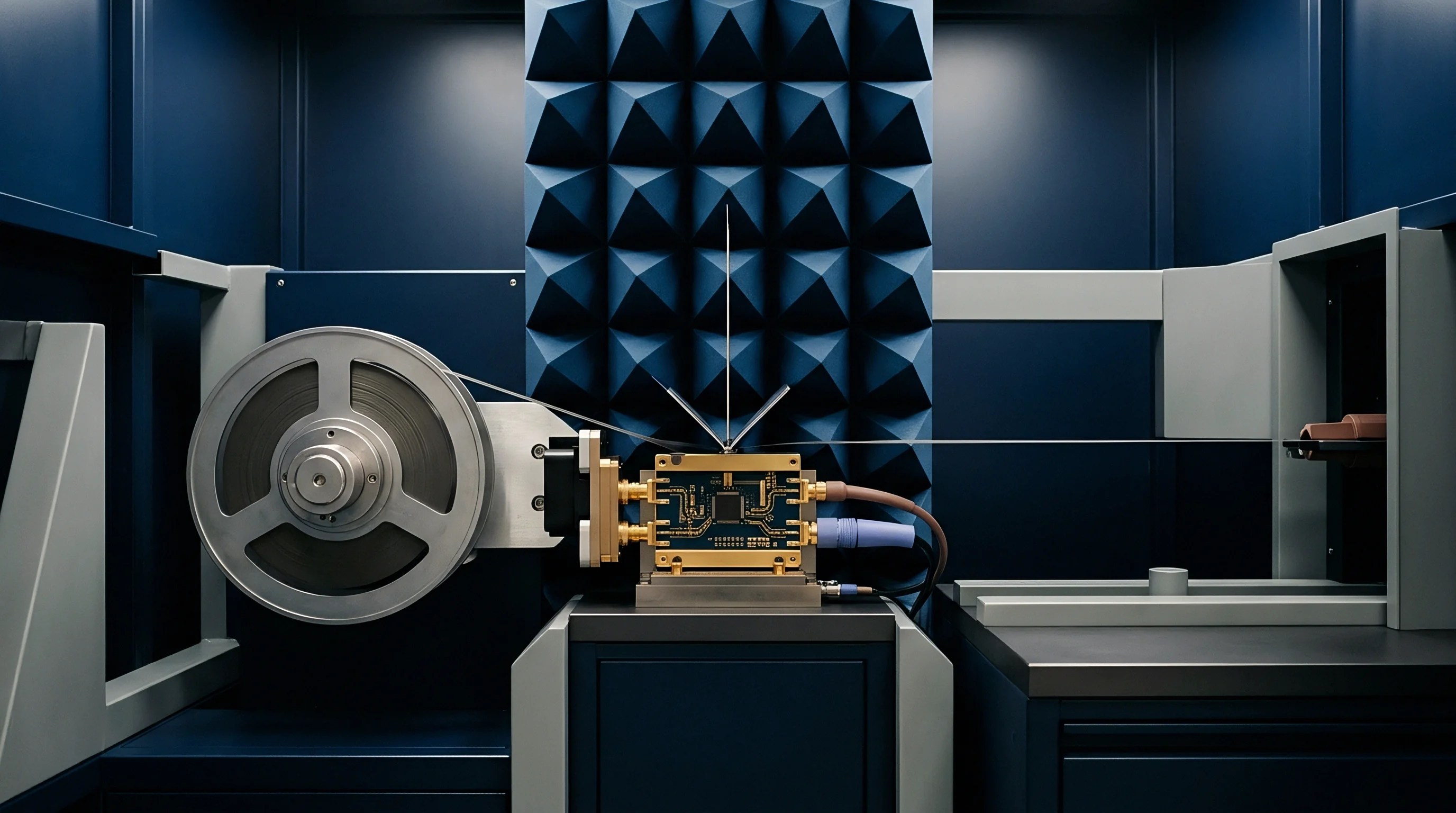
Precise extraction of S-parameters (S11 return loss, S21 insertion loss) at millimeter-wave frequencies requires Vector Network Analyzer (VNA) measurements paired with rigorous fixture de-embedding protocols. Standard coaxial-to-microstrip transitions introduce parasitic inductance and capacitance that mask the underlying performance of the substrate transmission line. Test engineers utilize Thru-Reflect-Line (TRL) or Short-Open-Load-Thru (SOLT) calibration coupons integrated directly onto the fabrication panel margins.
TRL calibration de-embeds fixture launches by measuring three distinct planar structures: a zero-length Thru connection, a high-reflection Reflect structure, and a Line structure whose electrical length differs from the Thru by 90 degrees at the center test frequency. TRL calibration moves the measurement reference planes directly to the edges of the substrate trace under test, eliminating launch reflections and isolating the intrinsic characteristic impedance, propagation constant, and dielectric loss tangent of the substrate layer.
IPC-6012 Class 3 specifications mandate dielectric thickness tolerances within plus or minus ten percent, bounding stripline deviation.
Substrate stackup qualification on production panels follows a sequential procedure to validate material compliance before component assembly.
- Extract panel edge coupons containing IPC-2441 TDR transmission line structures and VNA S-parameter calibration patterns.
- Perform picosecond-step TDR measurements across all controlled-impedance trace layers to verify characteristic impedance falls within specified tolerance bands.
- Connect calibrated Vector Network Analyzer probes to TRL de-embedding structures to extract true S11 return loss and S21 insertion loss curves.
- Pot coupon microsections in epoxy resin, section along the perpendicular trace axis, and polish the surface for optical metallographic inspection.
- Measure physical dielectric layer thickness, top trace width, bottom trace width, and copper plating thickness under a calibrated optical microscope to verify drawing compliance.

Time Domain Reflectometry and S-Parameter Coupon Testing
Specifying time-domain reflectometry coupon testing on every production panel isolates substrate thickness variations before component assembly. Panel coupons must accurately replicate the layer stackup, copper weight, prepreg selection, and trace geometry of the active circuit area. Fabricators often attempt to shrink coupon dimensions to preserve panel surface area for active boards, shortening coupon trace lengths below the minimum length required for stable TDR measurement.
Valid TDR impedance extraction requires a trace length long enough for the initial launch transient to settle completely before the pulse reaches the far end reflection. For a 20-picosecond rise-time instrument, the minimum valid test trace length is 50 millimeters. Shortening coupons to 20 millimeters forces the TDR measurement to record impedance during the inductive launch settling window, yielding false impedance readings that mask out-of-spec substrate stackup variations.
| Measurement Technique | Primary Parameter Extracted | Spatial Resolution | Production Inline Suitability | Governing Standard |
|---|---|---|---|---|
| Time-Domain Reflectometry (TDR) | Trace Impedance Profile Z0(x) | 1.5 to 3.0 mm | High (100% Panel Testing) | IPC-TM-650 2.5.5.7 |
| VNA S-Parameter (TRL De-embedded) | Return Loss S11, Insertion Loss S21 | Global Trace Segment | Moderate (Lot Sampling) | IEEE 287-2014 |
| Microsection Metallography | Physical H, W, T Geometries | Sub-micron Optical | Destructive (Panel Coupon) | IPC-TM-650 2.1.1 |
| Resonator Cavity Method | Bulk Dielectric Constant Er, Tan(delta) | Bulk Material Sample | Low (Incoming Raw Material) | IPC-TM-650 2.5.5.5 |
Cross-Sectional Microsectioning and Metallographic Audit
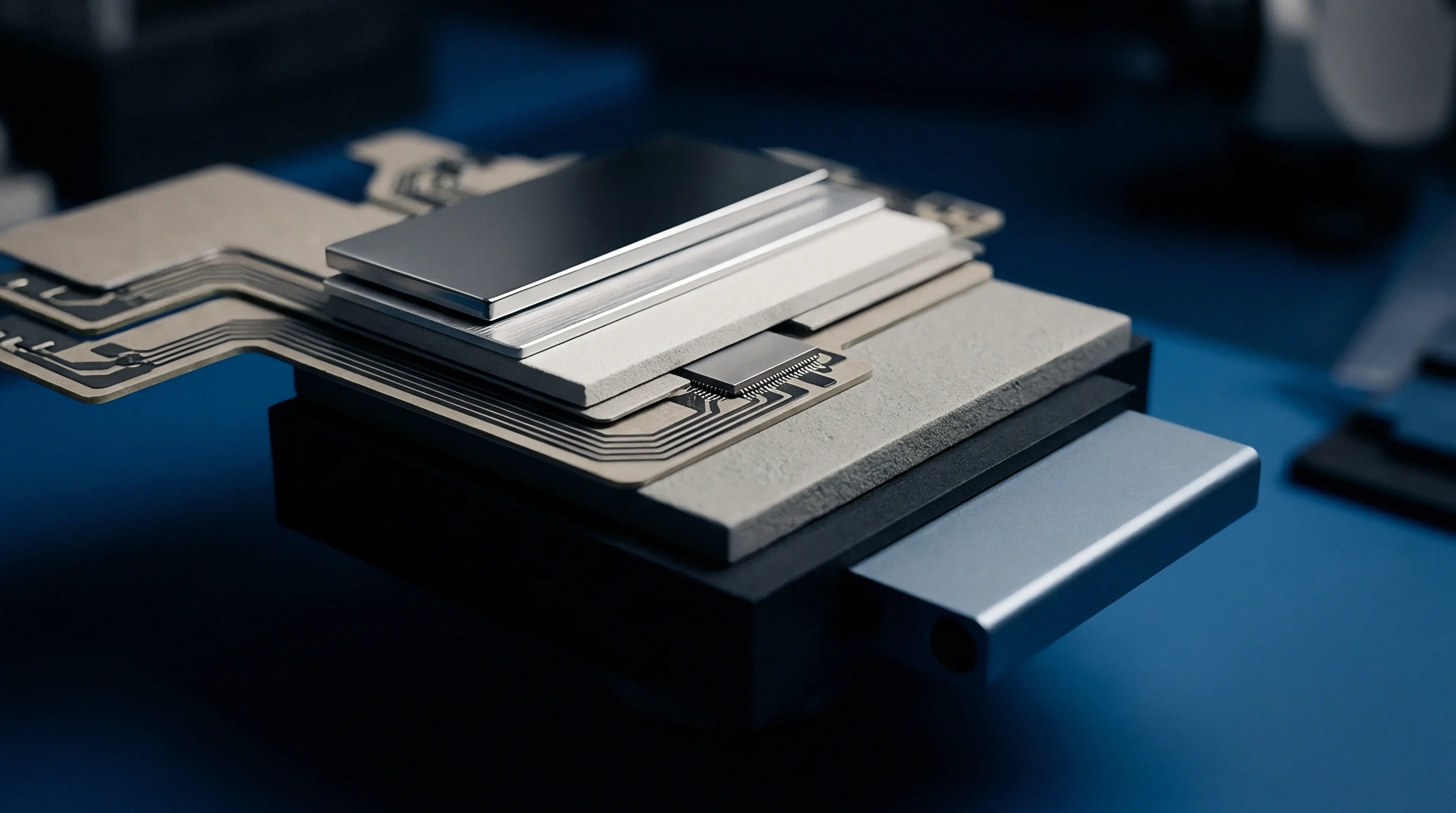
Destructive microsectioning provides optical verification of physical dimensions embedded within internal circuit board layers. Laboratory technicians cut panel coupons, encapsulate them in liquid epoxy resin, and grind the sample down to expose the transverse cross-section of signal traces. Polishing the cross-section with diamond paste enables high-magnification optical and Scanning Electron Microscope (SEM) inspection per IPC-TM-650 Method 2.1.1.
Microsection analysis quantifies exact physical dimensions: dielectric layer thickness H, bottom trace width W_bot, top trace width W_top, copper plating thickness, and plating barrel integrity inside microvias. Etch factor EF is calculated directly from microsection images using the formula:
EF = T / (W_bot – W_top)
Comparing physical microsection dimensions against TDR impedance measurements isolates whether impedance shifts stem from substrate raw material variations (incorrect Er or prepreg thickness H) or wet process chemical etch variations (incorrect trace width W or etch factor EF), directly safeguarding production schedules and non-refundable tooling investments.
Specifying IPC-6012 Class 3 coupon testing protocols binds the circuit fabricator to verified physical trace geometries prior to panel shipment.


Ledger
How financial risk is shared between module clients and board fabricators comes down to purchase contract specifics. Ordering boards based purely on mechanical dimensions without controlled-impedance acceptance criteria leaves buyers carrying the cost of RF mismatch failures. Standard shop defaults under IPC-6012 Class 2 allow plus or minus ten percent on dielectric thickness and plus or minus twenty percent on finished trace width ~ tolerances wide enough to sink high-frequency yields unless tight-control clauses are explicitly written into the contract.
Custom module programs requiring tight RF impedance control must contractually specify IPC-6012 Class 3 or explicit controlled-dielectric parameters. Standard manufacturing scope contracts assign dielectric lot qualification responsibility directly to the printed circuit fabricator. Moving from standard IPC-6012 Class 2 commercial tolerances to Class 3 tight-tolerance specifications increases raw bare-board purchasing costs by 15 to 30 percent.
However, this material premium is small compared to the scrap costs incurred when populated radio modules fail end-of-line RF return loss acceptance testing.
Commercial Risk Allocation in Printed Circuit Fabrication Contracts
Engineering scope agreements define the ownership boundary between design specifications and manufacturing deliverables. Turnkey module suppliers who accept design files without verifying substrate stackup tolerance limits often pass downstream yield loss costs back to the buyer through engineering change orders or piece-part price increases. Defining a complete design transfer package requires establishing precise tolerance boundaries for raw materials, copper processing, and layer registration.
Non-Recurring Engineering (NRE) tooling charges quoted by PCB fabricators cover photolithography tooling, lamination press programming, and impedance coupon test fixture configuration. When clients change substrate laminate specifications mid-program to fix unexpected RF mismatch issues, fabricators assess secondary NRE fees ranging from $2,500 to $8,000 per stackup iteration, while introducing four to six weeks of schedule delay. Specifying controlled-matrix microwave laminates like RO4350B, Rogers 4000 series, or Panasonic Megtron 6 during initial layout definition prevents costly re-tooling cycles.

Turnkey Sourcing Handover Package and Stackup Specifications
A comprehensive RF design handover package submitted to a fabricator contains precise manufacturing files beyond standard Gerber vectors. Modern fabrication transfer relies on IPC-2581 or Gerber X2 formats, which embed physical layer stackup definitions, material dielectric specifications, target impedance attributes, and copper foil profile requirements directly within the machine-readable dataset. Attaching explicit PDF stackup drawings to the RFQ package enforces legal compliance with specified dielectric tolerances.
The design transfer dossier must explicitly declare target impedance values, reference ground layers, allowed trace width variation limits, and mandatory coupon test structures. If a fabricator alters layer stackup spacing to adjust for internal prepreg inventory without client authorization, the handover package contract clauses provide clear legal grounds for panel rejection at the fabricator’s expense. The handover package must include signed material certification datasheets for every laminate and prepreg lot utilized in panel production.

Scrap Rate Arithmetic and Cost Trade-Offs of Microwave Laminates
Calculating the landed cost impact of substrate variance requires balancing raw laminate material costs against downstream PCBA yield loss. Standard FR-4 laminate material costs approximately $15 to $22 per manufacturing panel. Controlled-dielectric hydrocarbon ceramic laminates cost between $75 and $120 per panel.
High-performance PTFE laminates can exceed $250 per panel. For a high-density module design yielding 50 individual circuit boards per panel, raw FR-4 material adds $0.30 per board, whereas hydrocarbon ceramic material adds $1.80 per board.
Evaluate the scrap cost arithmetic of an assembled wireless module. Populating a single RF module with active transceivers, microcontrollers, passive components, and shielding cans costs $45.00 in total component and assembly labor. If an uncontrolled FR-4 substrate stackup causes an 18 percent failure rate at end-of-line RF return loss testing, the expected scrap cost per manufactured module is calculated as:
Scrap Cost per Unit = (Failure Rate Populated Board Cost) / (1 – Failure Rate)
Scrap Cost per Unit = (0.18 $45.00) / (1 – 0.18) = $9.88 per unit
Investing $1.50 per unit in premium controlled-matrix microwave laminates to eliminate substrate-induced mismatch failures reduces the downstream test failure rate to under one percent. Yield savings yield an immediate net cost reduction of $8.38 per shipped module, proving that raw material price savings are quickly wiped out by assembly scrap costs.
Engineering executives end up deciding whether the higher unit purchasing cost of tight-tolerance microwave laminates balances the financial exposure of downstream field recalls caused by uncharacterized dielectric drift.