Over the Air Receiver Sensitivity Loss Driven by Dynamic Antenna Impedance Detuning
Dynamic antenna detuning degrades over-the-air receiver sensitivity through both passive reflection loss and steep low noise amplifier noise figure expansion.


Grip
Dielectric loading shifts an antenna resonant frequency the instant a human hand, head, or metal bracket enters the reactive near-field zone. A radio frequency transceiver optimized for a nominal fifty-ohm terminal impedance experiences severe mismatch loss. Conducted sensitivity bench figures fail to predict this loss because testing cables maintain fifty ohms resistive impedance regardless of the physical surroundings.
In field deployments, the antenna terminal impedance departs from the center of the Smith chart. The impedance vector migrates along constant conductance and resistance contours, dropping return loss from eighteen decibels down to two decibels or less. Mismatches reflect incoming signal power.
Near-field interactions alter the complex input impedance Z_in = R_in + jX_in by introducing parasitic capacitance and dielectric loss. High-permittivity human tissue exhibits a relative dielectric constant between thirty and fifty-five across sub-gigahertz and 2.4 gigahertz frequencies, alongside significant conductivity. This biological volume pulls electromagnetic energy into lossy heating while dragging the electrical antenna resonance lower in frequency.
An antenna tuned for 868 megahertz in free air shifts toward 815 megahertz under direct palm touch. For a narrow-band long range system or an LTE Cat-M1 channel, this frequency translation shifts the operational transmission channel completely outside the antenna operating bandwidth.
A three-picofarad human palm shunt capacitance drags antenna resonance downward by eighty megahertz at 2.4 gigahertz, introducing twelve decibels of mismatch loss at the receiver input.
Losses multiply across the receiver chain. The signal delivered to the receiver low noise amplifier drops proportionally to the mismatch factor M = 1 – |Gamma|^2, where Gamma represents the complex voltage reflection coefficient. When an antenna operating at 915 megahertz presents a voltage standing wave ratio of 8.0:1 under hand loading, Gamma reaches approximately 0.78, yielding a mismatch factor of 0.39.
This reflection directly introduces 4.1 decibels of insertion loss before the signal enters the silicon front-end package.

Environmental Dielectric Loading
Proximity to real-world objects alters the reactive energy distribution stored within the radian sphere of the radiator. When water containers, moist soil, structural concrete, or human flesh press against an enclosure, the boundary condition for Maxwell curl equations changes instantly. The phase velocity of the guided wave drops, shrinking the apparent electrical wavelength and transforming inductive trace sections into capacitive elements.
Return loss drops below acceptable limits.
Plastic housings made from polycarbonate or acrylonitrile butadiene styrene impose an initial static frequency pull, which bench engineers correct using fixed lumped-element matching circuits. Dynamic loading introduces transient impedance states that no single fixed passive circuit can accommodate. A handheld scanner resting on a metal workbench presents a near-short-circuit impedance vector.
The same unit carried by a worker wearing leather gloves presents high-impedance parallel loading. Field environments alter dielectric boundaries.
The Smith Chart Displacement Trajectory
Impedance excursions follow distinct trajectories on the complex reflection plane depending on the radiator architecture. Inverted-F antennas, ceramic patch elements, and monopole stubs exhibit divergent displacement paths under identical physical proximity disturbances. A planar inverted-F antenna loaded by a thumb shifts along a capacitive arc toward the lower hemisphere of the Smith chart.
A ceramic chip antenna exhibits strong dielectric coupling that pulls its inductive loop into over-coupled resonance orbits.
Phase angle rotations between the antenna feed point and the transceiver input pin further alter the apparent load. A two-centimeter microstrip feed trace on standard FR-4 substrate introduces significant phase transformation at 2.4 gigahertz. A load that appears as eight ohms resistive at the antenna feed pin transforms into a complex high-impedance reactive state at the low noise amplifier input pin.
This phase rotation changes how the semiconductor active devices respond to the incoming power level.

Voltage Standing Wave Ratio Extremes
Extreme detuning drives the voltage standing wave ratio beyond standard operating thresholds. Normal factory alignment targets an input voltage standing wave ratio below 1.5:1 across the operating channel, corresponding to less than 0.18 decibels of reflection loss. In practical handheld and body-worn deployments, the standing wave ratio routinely climbs past 6:1, reaching 12:1 during complete device encirclement by human fingers.
At 12:1, ninety percent of the available incoming signal power reflects off the receiver front-end interface.
Deploying wireless tracking modules without accounting for dynamic reflection extremes produces erratic coverage dropouts, unacknowledged transmissions, and dead spots across operating environments where line-of-sight signal strength ought to sustain clean communication links.

Stage
Silicon active stages react to off-nominal source impedances through non-linear noise generation rather than passive attenuation alone. The noise factor of a receiver low noise amplifier depends directly on the source admittance presented at its input terminal. Semiconductor designers characterize this interaction through source noise circles defined by four noise parameters: minimum noise figure F_min, equivalent noise resistance R_n, and the complex optimum source admittance Y_opt.
When the antenna impedance moves away from the optimum source impedance, the amplifier noise figure increases independently of the passive reflection loss. The noise figure climbs rapidly.
Conducted receiver sensitivity figures stated on module datasheets assume a clean fifty-ohm resistive source. Under this idealized condition, the internal low noise amplifier operates near its designated noise minimum, delivering sensitivities such as -148 dBm for LoRa at spreading factor 12, -97 dBm for Bluetooth Low Energy at one megabit, or -105 dBm for NB-IoT. When the antenna detunes, the source impedance seen by the silicon stage swings wildly.
The low noise amplifier shifts along steep noise figure contours, increasing its internal noise contribution by three to eight decibels. Phase rotations distort noise parameters.
A receiver low noise amplifier presenting an optimum noise match at fifty ohms suffers a five-decibel noise figure degradation when dynamic loading drives the antenna input impedance to ten ohms.
The total degradation in receiver sensitivity equals the sum of the passive mismatch loss and the excess noise figure penalty. An antenna presenting a 6:1 voltage standing wave ratio produces approximately 3.1 decibels of passive reflection loss. If that specific complex impedance shifts the active stage two decibels away from its optimum noise circle, the total receiver sensitivity degrades by 5.1 decibels.
An extra five decibels of sensitivity loss cuts the effective operating range in half under free-space propagation conditions.

Low Noise Amplifier Noise Circles
Noise circles represent geometric loci on the Smith chart where the stage noise figure remains constant. At the center of these concentric contours sits Gamma_opt, the reflection coefficient delivering minimum noise contribution. Semiconductor architectures such as complementary metal-oxide-semiconductor and silicon-germanium heterojunction bipolar transistors display tight, densely packed noise contours.
Gain circles run obliquely across noise circles. The impedance that maximizes power transfer does not match the impedance that minimizes active noise figure. A dynamic impedance swing can push the system toward an unstable region of the amplifier stability circles, inducing regenerative feedback, spurious oscillations, or intermodulation distortion in the presence of out-of-band blocking signals.
Input Impedance Noise Factor Derivation
Mathematical modeling of front-end noise behavior illustrates how source admittance shifts degrade receiver operation. The stage noise factor obeys the classical expression:
F = F_min + (R_n / G_s) |Y_s – Y_opt|^2
In this formulation, Y_s = G_s + jB_s represents the actual source admittance presented by the detuned antenna and matching components, while Y_opt = G_opt + jB_opt represents the optimum admittance. When dynamic loading reduces the source conductance G_s toward zero, the fraction R_n / G_s expands rapidly. Small deviations between actual susceptance B_s and optimum susceptance B_opt produce quadratic growth in the total noise factor.
Fixed matching circuits remain static.
| Source Impedance (Ohms) | VSWR | Mismatch Loss (dB) | Noise Figure Adder (dB) | Total Sensitivity Loss (dB) |
|---|---|---|---|---|
| 50 + j0 | 1.0:1 | 0.00 | 0.00 | 0.00 |
| 25 – j15 | 2.3:1 | 0.76 | 0.85 | 1.61 |
| 15 + j30 | 4.2:1 | 2.10 | 1.95 | 4.05 |
| 8 – j20 | 7.1:1 | 3.62 | 3.40 | 7.02 |
| 5 + j5 | 10.2:1 | 4.98 | 5.20 | 10.18 |
Front End Degradation States
The operational failure modes created by dynamic antenna mismatch fall into several physical categories:
- Noise Figure Collapse occurs when the source impedance strays into high-noise Smith chart coordinates, drowning low-amplitude incident packets beneath active silicon thermal noise.
- Linearity Degradation develops as mismatch phase rotations lower the third-order input intercept point, allowing co-located transmitters to create destructive intermodulation products.
- Bandpass Skewing happens when the antenna terminal reactance interacts with front-end surface acoustic wave filters, shifting filter passband corners into rejection skirts.
- Gain Compression arises from standing wave voltage peaks driving the initial amplification transistor into premature saturation under modest interference levels.
Active stages maintain optimal signal-to-noise ratios only while the source impedance stays confined within the inner noise circle boundary.


Budget
Link calculations routinely overestimate field reach by relying on conducted sensitivity figures published in silicon datasheets. A wireless module specifying -120 dBm conducted receiver sensitivity assumes lossless, non-reactive energy transfer into the receiver pin. Over-the-air performance diverges from conducted metrics because radiation efficiency and impedance match fluctuate dynamically in field conditions.
Total Isotropic Sensitivity characterizes true over-the-air receiver capability by integrating sensitivity across an entire three-dimensional spherical coordinate system. Conducted measurements hide field degradations.
Total Isotropic Sensitivity incorporates antenna efficiency alongside receiver noise figure. The metric represents the integrated sphere power level at which packet error rate reaches a designated threshold, such as 10 percent for Long Range or 0.1 percent for Bluetooth Low Energy. If an antenna exhibits negative three decibels of radiation efficiency in free air, a radio with -100 dBm conducted sensitivity yields a Total Isotropic Sensitivity of -97 dBm.
Hand proximity worsens this figure by introducing dielectric dissipation and mismatch reflection, frequently shifting Total Isotropic Sensitivity to -85 dBm or worse. Link budgets collapse without margin.
A LoRa sensor operating with a twenty-decibel link margin loses connectivity entirely when human proximity induces twelve decibels of over-the-air sensitivity loss across non-line-of-sight paths.
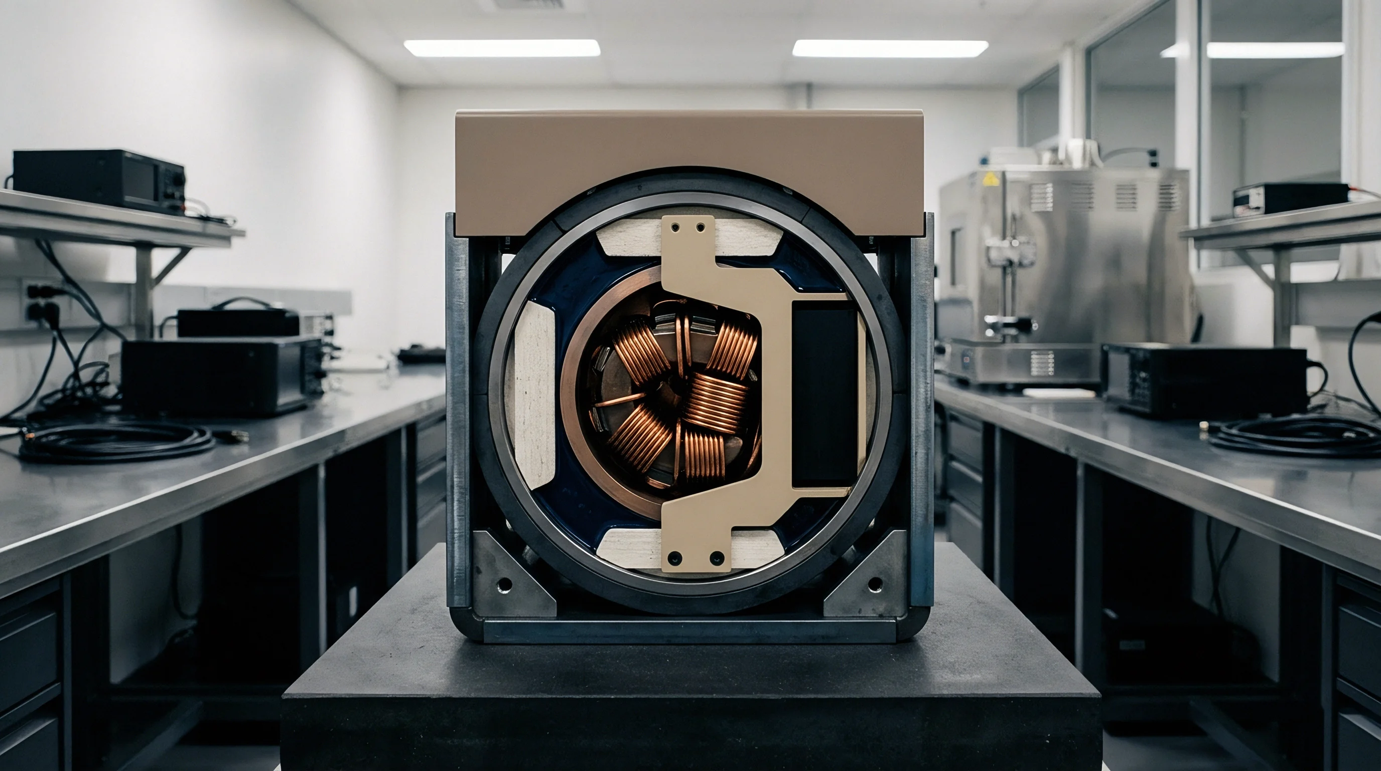
Measuring this degradation requires specialized over-the-air test ranges. Anechoic chambers equipped with multi-axis positioning systems evaluate receiver sensitivity while biological phantoms simulate real-world mechanical loading. Hand phantoms made of carbon-loaded silicone mimic human hand dielectric properties, establishing repeatable impedance detuning conditions across frequency bands.
Hand capacitance absorbs radiated field energy.

Conducted Sensitivity versus Isotropic Sensitivity
Conducted sensitivity evaluates receiver silicon behind a fifty-ohm coaxial cable, while over-the-air sensitivity captures complete physical reality. Silicon suppliers guarantee conducted sensitivity within tight production tolerances of plus or minus one decibel. In contrast, over-the-air Total Isotropic Sensitivity spans a wide distribution across identical boards due to assembly tolerances, enclosure proximity, and user handling postures.
The gap between conducted sensitivity and Total Isotropic Sensitivity represents the implementation penalty. In industrial Internet of Things tracking designs, this penalty commonly exceeds ten decibels under severe dynamic detuning. An engineer who calculates link margin using conducted numbers risks a field failure rate exceeding twenty percent during humid conditions or dense physical contact.

The Chamber Measurement Procedure
Quantifying dynamic over-the-air sensitivity loss follows a strict sequential measurement procedure within an anechoic chamber:
- Mount the unit under test onto a low-permittivity dielectric turntable at the center of the quiet zone.
- Establish an active over-the-air communication link with the communication tester using the selected frequency and modulation profile.
- Step the turntable azimuth and elevation angles through fifteen-degree increments across 360 degrees of horizontal and 180 degrees of vertical rotation.
- Sweep downlink signal generator output power downward at each position until packet error rate crosses the specified limit.
- Repeat the complete spatial spherical sweep with a standardized anthropomorphic hand phantom attached directly to the product enclosure.
- Integrate the measured sensitivity points across the complete sphere surface to calculate the Total Isotropic Sensitivity delta between loaded and free-space states.
| Protocol | Band | Conducted Sens. (dBm) | Free Space TIS (dBm) | Hand Loaded TIS (dBm) | Total OTA Loss (dB) |
|---|---|---|---|---|---|
| BLE 1 Mbps | 2.4 GHz | -96.0 | -92.5 | -81.0 | 11.5 |
| Wi-Fi 6 (MCS0) | 2.4 GHz | -98.0 | -94.0 | -83.5 | 10.5 |
| LoRa (SF10) | 868 MHz | -132.0 | -128.0 | -114.5 | 13.5 |
| LTE-M (HD-FDD) | B20 (800 MHz) | -106.0 | -101.5 | -89.0 | 12.5 |
| NB-IoT | B8 (900 MHz) | -114.0 | -109.0 | -95.0 | 14.0 |

Total Isotropic Sensitivity Degradation across Protocols
Sub-gigahertz protocols like LoRa and NB-IoT suffer greater impedance detuning penalties than 2.4 gigahertz links when human tissue enters the reactive field. Because sub-gigahertz antennas rely on physical dimensions proportional to longer wavelengths, the ground plane of the printed circuit board forms a substantial portion of the radiating structure. A hand gripping an entire device shunts current across the ground plane, shifting resonance substantially.
Battery drain accelerates under repeat packets.
At 2.4 gigahertz, antenna dimensions remain compact, concentrating reactive fields closer to the antenna element. While biological tissue absorbs 2.4 gigahertz electromagnetic energy through bulk water polarization, the relative frequency pull represents a smaller percentage of overall channel bandwidth compared to narrow sub-gigahertz channels.
Suppliers routinely dismiss field sensitivity complaints by claiming that laboratory conducted test benches verify full compliance with published module specifications.

Carrier
Cellular carriers enforce stringent over-the-air receiver performance standards to protect base station capacity and maintain reliable cell-edge handovers. Organizations such as PTCRB and CTIA set mandatory Total Isotropic Sensitivity thresholds that cellular modules must pass inside certified testing chambers before carrier activation is permitted. Dynamic impedance detuning poses a direct commercial barrier during certification.
A device passing conducted verification easily fails carrier Total Isotropic Sensitivity limits by five decibels the moment a battery phantom or hand fixture attaches to the enclosure. Carrier certification demands radiated audits.
When an LTE-M or NB-IoT device experiences receiver sensitivity degradation in the field, base stations compensate by commanding higher transmission power and increasing down-link repetition rates. Repetitions consume network time slots, raising carrier operational overhead while exhausting the end device battery. A device engineered for a ten-year operational life on an internal battery can deplete its energy reserves in under twenty-four months due to repeated downlink acknowledgments and signal recovery loops caused by poor over-the-air sensitivity.
Under PTCRB test specification 2.2, a cellular device that fails Total Isotropic Sensitivity limits by a single decibel faces immediate rejection from carrier certification rosters.
To overcome dynamic mismatch, modern cellular and multi-band IoT designs incorporate dynamic impedance matching circuits. Dynamic tuners leverage micro-electro-mechanical systems switches or barium strontium titanate variable capacitors to shift the matching circuit reactances in real time. These components restore the impedance presented to the low noise amplifier toward fifty ohms, mitigating both passive reflection loss and amplifier noise figure expansion.

Protocol Error Ceilings and Packet Loss
Different protocols exhibit varied tolerance profiles when dynamic antenna mismatch degrades the receiver signal-to-noise ratio:
- Bluetooth Low Energy uses short transmission packets and adaptive frequency hopping, but suffers severe connection dropouts when detuning creates nulls across advertising channels 37, 38, and 39.
- Wi-Fi Systems step down modulation and coding schemes toward robust binary phase-shift keying modes, preserving the link at the cost of airtime congestion and increased power consumption.
- LoRaWAN Nodes rely on fixed spreading factors set by Adaptive Data Rate algorithms, which can fail to adjust if downlink signaling packets are lost to severe receiver detuning.
- Cellular NB-IoT relies on massive downlink subframe repetition, burning battery reserve capacity to decode signal blocks that drop below the noise floor.
Dynamic Impedance Tuners and Switched Matching
Closed-loop and open-loop antenna tuners offer distinct architectural trade-offs for embedded transceivers. Open-loop tuners read transmit power detector registers or proximity sensor inputs to select predetermined capacitance states from a lookup table. Closed-loop tuners incorporate directional couplers and phase detectors to measure reflected power directly at the antenna feed, adjusting shunt reactances until return loss improves.
Aperture tuners preserve radiation resistance.
Aperture tuning alters the electrical length of the antenna element by switching discrete capacitors or inductors across dedicated antenna loading ports. Aperture tuning preserves radiation efficiency better than impedance matching at the feed line, because it alters the current distribution along the radiator itself. Feed line impedance tuners correct the match seen by the transceiver, but cannot recover radiation efficiency lost to physical dielectric dissipation.
| Tuning Architecture | BOM Adder (USD) | PCB Area (mm²) | TIS Recovery (dB) | Power Consumption |
|---|---|---|---|---|
| Fixed LC Ladder Match | 0.00 | 6.0 | 0.0 (Baseline) | Zero |
| Switched RF PIN Diodes | 0.28 | 14.0 | 2.5 – 4.0 | 5 – 15 mA (Continuous) |
| RF MEMS Switch Array | 0.65 | 8.5 | 4.0 – 7.5 | 10 – 50 µA (Static) |
| BST Varactor Shunt | 0.85 | 10.0 | 3.5 – 6.5 | 20 – 80 µA (Static) |
| Closed-Loop Directional Tuner | 1.45 | 22.0 | 6.0 – 9.0 | 1.5 – 3.5 mA (Active) |
Carrier Certification Margin Deficits
Passing carrier certification demands careful design margin over minimum regulatory thresholds. A typical operator requires an LTE Cat-M1 receiver Total Isotropic Sensitivity better than -99.5 dBm on Band 4 and -96.5 dBm on Band 13. A module boasting a conducted sensitivity of -106 dBm leaves less than ten decibels of budget for combined antenna inefficiency, enclosure loss, and hand loading.
PTCRB qualification guidelines dictate that cellular devices failing anthropomorphic hand phantom tests cannot receive operational acceptance certificates until board respins demonstrate compliance.


Settlement
Procuring wireless modules based purely on silicon pricing creates severe downstream financial exposures during physical system qualification. Module purchase agreements frequently omit over-the-air receiver guarantees, leaving the buyer entirely liable for link margin deficits caused by environmental detuning. A module bill of materials saving thirty cents can easily trigger a twenty-thousand-dollar chamber retest fee alongside four months of tooling modifications when the product fails operator radiated sensitivity audits.
Supply agreements must specify strict impedance tolerance limits and receiver noise figure boundaries across mismatched source states. Request-for-proposal documents that solely demand conducted sensitivity figures allow module suppliers to deliver silicon optimized with aggressive, narrow-band internal matches. These matches degrade rapidly under slight reactive loading.
Specifying maximum noise figure expansion under a 4:1 voltage standing wave ratio across all phase angles forces suppliers to deliver robust, wideband low noise amplifier front ends.
Warranty allocations between original design manufacturers and module suppliers require quantifiable boundaries. When an asset tracker experiences intermittent communication loss in customer hands, field service teams often replace units unnecessarily, assuming battery or firmware failures. Pinpointing dynamic antenna detuning as the root cause demands calibrated over-the-air return loss loggers or specialized diagnostic firmware that tracks automatic gain control states and packet drop ratios during operational motion.
Hardware Procurement and Tuner Bill of Materials
Factoring dynamic tuning components into early product accounting models protects project profitability. Adding an aperture tuning switch and associated passives increases module unit costs by sixty to eighty cents. This investment eliminates the need for expensive high-gain external antenna accessories or costly post-production firmware workarounds that shorten battery life.
Procurement teams must evaluate total cost per delivered message across product lifespans. If antenna detuning increases cellular packet retransmissions from two percent to eighteen percent, cellular data overage fees quickly outstrip the initial capital cost of an integrated antenna tuner circuit.

RFQ Specifications for Impedance Variance
Drafting precise sourcing requirements prevents downstream technical disagreements. Commercial RFQs should define receiver sensitivity requirements across a full 360-degree phase sweep at defined standing wave ratios. Requiring suppliers to deliver low noise amplifier noise parameter datasets enables system designers to simulate over-the-air performance before committing to volume tooling.
Verification clauses must mandate chamber testing with standardized anthropomorphic phantoms representing the end-use operational posture. Skipping phantom verification during qualification guarantees that impedance mismatch problems will emerge only after volume production begins.

Field Return Liability Clauses
Contracts governing wireless hardware delivery must explicitly define performance failure criteria under real-world usage postures. Incorporating receiver Total Isotropic Sensitivity thresholds into incoming quality acceptance sampling establishes clear commercial remedies when delivered lots display excessive front-end sensitivity dispersion.
How component suppliers and device manufacturers will equitably split warranty costs when environmental detuning causes intermittent packet failure across dense industrial environments remains an open contractual challenge.